The previous formulas I proposed (based on fitting the timings of the play to a normal distribution) become, simpler, more accurate, and faster to calculate if one uses the exact timing of each hit instead of the judgment counts.
How would the scoring system work:
1) Take the exact error of each note that was hit. For LN releases, divide it's error by x1.5 (to account for the fact that it's harder to time releases than hits), the multiplier could be adjusted to other value. Do not consider hits/releases that were hit in their "Miss" timing window.
Take the sum of the squares of those errors (that value will be referred as "s"), and the count of the hits and releases that weren't misses (referred as "k").
2) Count the amount of misses notes and releases (referred as "m").
3) With that information, calculate the Normal Distribution with zero mean that fits the data the best, obtaining the standard error Sigma (details of the calculation below).
4) Use a scaling function that maps that standard error to a score. A good choice for this function is, for Sigma measured in ms:
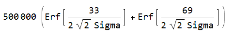
Erf is the Error Function. In the case Sigma is zero (which is only possible with a perfect play, which should be almost certainly impossible), then the score is 1 million.
For EZ/HT, for balance, it would be best if they don't change the timing window for 50s nor the timing window for Misses. That way, they can't have an effect on score, they become merely cosmetic (changing the distribution of the judgments during the play). DT/HT shouldn't change the timing window of 50s and Misses either (besides scaling to make internal clocks match real time, like it is done currently). To make scores with different ODs in the same map be directly comparable, those timing windows shouldn't change either (this way, OD becomes merely cosmetic as well while playing).
How would the scoring system work:
1) Take the exact error of each note that was hit. For LN releases, divide it's error by x1.5 (to account for the fact that it's harder to time releases than hits), the multiplier could be adjusted to other value. Do not consider hits/releases that were hit in their "Miss" timing window.
Take the sum of the squares of those errors (that value will be referred as "s"), and the count of the hits and releases that weren't misses (referred as "k").
2) Count the amount of misses notes and releases (referred as "m").
3) With that information, calculate the Normal Distribution with zero mean that fits the data the best, obtaining the standard error Sigma (details of the calculation below).
4) Use a scaling function that maps that standard error to a score. A good choice for this function is, for Sigma measured in ms:
Erf is the Error Function. In the case Sigma is zero (which is only possible with a perfect play, which should be almost certainly impossible), then the score is 1 million.
For EZ/HT, for balance, it would be best if they don't change the timing window for 50s nor the timing window for Misses. That way, they can't have an effect on score, they become merely cosmetic (changing the distribution of the judgments during the play). DT/HT shouldn't change the timing window of 50s and Misses either (besides scaling to make internal clocks match real time, like it is done currently). To make scores with different ODs in the same map be directly comparable, those timing windows shouldn't change either (this way, OD becomes merely cosmetic as well while playing).
Calculating the Standard Error "Sigma"
The variables are:
s = Sum of the squares of the timing errors of hits/releases that weren't a Miss. (Releases with errors scaled by a constant)
k = Count of hits/releases that weren't a Miss.
m = Count of Misses.
T = Upper limit of the timing window for a 50, in ms.
Case with no Misses
Sigma is simply
Case with Misses
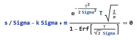
Sigma is the positive number that solves the equation:
The equation doesn't have a simple closed form solution, but it can be easily solved numerically with Newton's Method (since the function to find a root for is convex and monotonic).
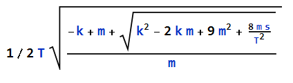
A first approximation of Sigma (that always is smaller than the real solution) is:
With BS = T/Sigma.
Function to find the root for: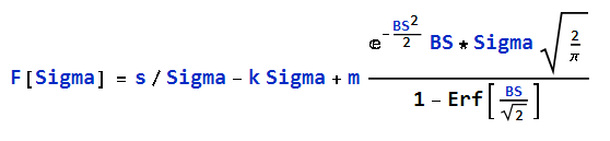
It's derivative: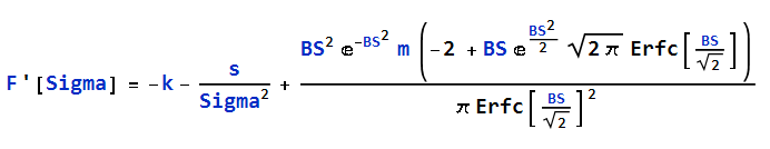
Note: Because of numerical errors while using double floating-point numbers to calculate the functions, for high values of BS, it's more accurate to use a series expansion near Sigma=0, instead of attempting to calculate their values with the exact formulas.
If BS > 7, then: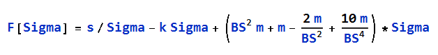
If BS >20, then: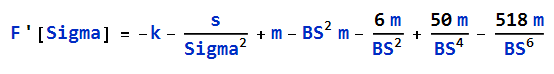
The, starting with the initial approximation for sigma, iterate with Newton's Method until F[Sigma] is small:
Sigma[n+1] = Sigma[n] - F[Sigma[n]] / F'[Sigma[n]]
Testing this algorithm, it takes about 0.8ms in average to find an accurate value for Sigma (with an absolute error of 10^(-7)).
s = Sum of the squares of the timing errors of hits/releases that weren't a Miss. (Releases with errors scaled by a constant)
k = Count of hits/releases that weren't a Miss.
m = Count of Misses.
T = Upper limit of the timing window for a 50, in ms.
Case with no Misses
Sigma is simply
Case with Misses
Sigma is the positive number that solves the equation:
The equation doesn't have a simple closed form solution, but it can be easily solved numerically with Newton's Method (since the function to find a root for is convex and monotonic).
A first approximation of Sigma (that always is smaller than the real solution) is:
With BS = T/Sigma.
Function to find the root for:
It's derivative:
Note: Because of numerical errors while using double floating-point numbers to calculate the functions, for high values of BS, it's more accurate to use a series expansion near Sigma=0, instead of attempting to calculate their values with the exact formulas.
If BS > 7, then:
If BS >20, then:
The, starting with the initial approximation for sigma, iterate with Newton's Method until F[Sigma] is small:
Sigma[n+1] = Sigma[n] - F[Sigma[n]] / F'[Sigma[n]]
Testing this algorithm, it takes about 0.8ms in average to find an accurate value for Sigma (with an absolute error of 10^(-7)).