Almost wrote:
Full Tablet wrote:
If there is no correlation, it is almost impossible to obtain a value of r<=-0.11 with a large sample. When there is no correlation, as you increase the sample size, |r| tends to approach 0, so it is not true that as you increase the sample size you are more likely to find a statistically significant correlations when there are actually none.
As I said mathematically, yes there is a correlation but the issue is whether such a correlation is practically relevant. The amount of variance in the plot says no. Essentially, this correlation is purely fit to noise.
You are just repeating your points here. As I said earlier, there are conclusions that are practically relevant even if the correlation found is weak. For example, we can conclude that the correlation is not null nor positive (so it is not reasonable to increase your average playcount expecting to get pp more efficiently, and "never retry" is likely bad advice if one seeks to gain pp efficiently), we can also conclude that the correlation is weak, so we can't confidently predict the outcome based on the variables (in other words, "Your mileage might vary").
You seem to be confusing measurement noise with inherent noise in the data; measurement noise does weaken some inferences you might make from the data (but not all inferences, such as the existence of correlation, except when the noise itself is correlated), inherent noise (noise we would obtain even if the measurements are perfect) does not make the inferences less reliable, it just makes predictions less reliable.
Almost wrote:
Full Tablet wrote:
Yes, due to not having much data outside the 100-250 play-length, we can't infer much about the effect of play length on improvement rate outside that play-length range (but still, we do have information about the effect inside the range).
And you're just going to infer that the correlation is the same?? Not that it matters though since there's just way too much variance in the data.
I am not inferring that the correlation is the same outside the points we have more data on. I am saying that we can't infer as confidently outside the range as we would do inside the range.
Almost wrote:
Full Tablet wrote:
If we sampled again with more data outside that range, and found that the correlation is weaker across all the range, then we would need to check for non-linear relationships between the variables. For example, it is possible that there is a bitter spot in play-length (for small play-lengths, increases of play-length tends to decrease improvement rate, and for big play-lengths, increases of play-length tends to increase improvement rate).
Again, there's really no point in pontifiyng things outside the realm of possibility. It's realistically impossible to gather this data that's actually very clean.
Acknowledging what we don't know is also important. If we aren't able to know about something, we should take into consideration all possibilities about it (which is not the same as assuming that one of the possibilities is true, which would be something obviously wrong to do).
Almost wrote:
Correlation coefficient calculation is based off the least squares method which basically finds the line of best fit for a given set of data points. Since the distribution of this data is skewed towards the lower improvement ranges for basically all play lengths and there also being lack of data for the higher play lengths, there is a lower representation of the higher rates of improvement in the high play lengths. Simply put, since the distribution of the data is like below, if you were to have more data for the higher play lengths, you'd likely just get a uniform plot without any real change in the rate of improvement vs average play length since the distribution is pretty linear no matter the play length.
Do you think that the sampling process was skewed towards selecting points that have low improvement ranges? The fact that the data obtained has a skewed distribution doesn't mean that the sample is biased, as far as we know, that skew seems to be a characteristic of the population.
Also, if the distribution of the independent variable in the data is skewed towards lower values, it is not true that you should expect getting a false negative slope in the linear regression of the data.
Example:
Suppose that in the population, there is an inherent randomness in the value obtained in the dependent variable for each point in the independent variable, with the randomness following a skewed distribution.
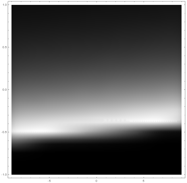
(The closer the point is to white, the more probable is to obtain that value). The best possible prediction of y given x is a linear function y(x) = 0.01x, and the true correlation between the two variables is r=0.115216.
Now, we do a sample that is very skewed towards taking points with low values of x:
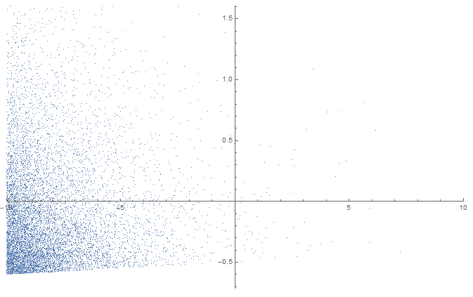
This sample has a linear regression of y(x) = 0.0000122334 + 0.0100465x, and r=0.115216, which is pretty close to the ideal parameters. If we repeat this skewed sampling several times we obtain similar results. There is no tendency to find slopes when we shouldn't with the skewed sampling.
Another example:
Suppose that the population follows this distribution for each x:
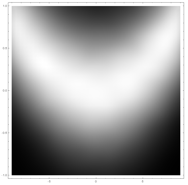
Which has an ideal prediction function y(x)=0.01x^2, and r^2=0.258148. Attempting a linear regression with a sample of this population would fail with r very close to 0.
Now let's take a very skewed sample:
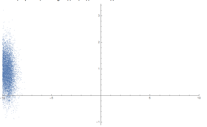
A linear regression gives y(x)=0.33314 -6.47732*10^-6 x, with r=-0.0000643552 (so it fails).
A quadratic regression gives y(x)=0.00303735 -6.47732*10^-6 x+0.00990298 x^2, with r^2=0.258148. So even a sample this skewed reproduces the non-linearity of the population.
Abraker wrote:
Full Tablet, can you post density scatter plots with contours for the results?
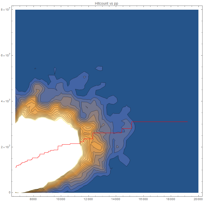
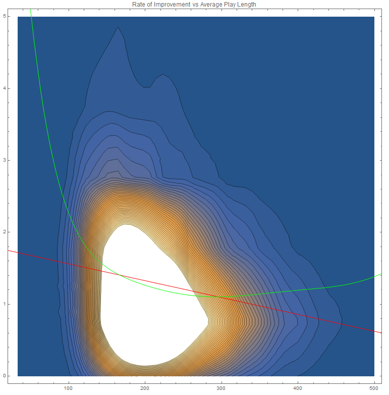
Here it is (using a Gaussian kernel).
I also included a high-degree (7) polynomial regression curve, which has r^2=0.0225744 (|r|=0.150248, better than the one in the linear model with r = -0.116515), which is significant at a significance level of 1%. This curve is better for predicting rate of improvement given the average hitcount in the white area of the graph (where we have the most information), but high-degree curves are worse at extrapolating compared to linear curves, and the low value of r^2 indicates that the predictions are still not reliable.
Doing a F-test to check whether or not the high-degree polynomial model fits the data significantly better than the linear model (null hypothesis: high-degree polynomial model does not provide a significantly better fit than the linear model), we conclude that the polynomial model is significantly better with a false-rejection probability less than 1%.