Props to all the effort put into this, but I still think not retrying is a better way to improve at the game. Remember this: PP does not measure all types of skills in osu!
forum
The reason why "never retry" is (probably) bad advice
posted
Total Posts
45
My two cents in this matter: i think that retrying ability should be used smartly. For example retrying a map 100 times just to get an proper fc is not a smart play. To retry a map 5 times to get down a certain pattern would be a better use. But perhaps the best use case is just where you know you should have done better. The first time you don't do very well for example environmental reasons, and then your next play is, indeed, a better play than your last. That would be a good use case for a retry. But indeed, the majority of your plays should be from new maps that are a little above your comfort zone
I repeated the analysis with data extracted today.
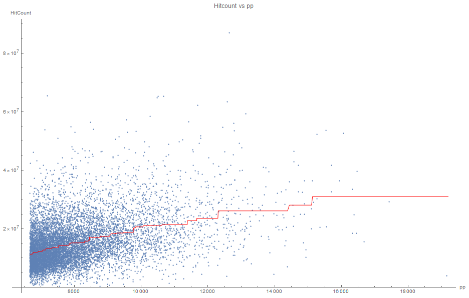
One problem with defining the rate of improvement as pp/hitcount is that, as seen in the data, the expected amount of pp given a certain hitcount is not linear, but rather roughly a monotonically increasing quasi-convex function. This means that the pp/hitcount value tends to be higher when the player is higher ranked (which contradicts the hypothesis previously made that low-ranked players tend to show higher rates of pp/hitcount). The solution given by Railey2 is filtering to narrowed ranges of ranking (which works is the range is small enough to make the relationship between pp and hitcount roughly linear).
Instead, I define rate of improvement as the expected hitcount given the amount of pp of the player, divided by the hitcount of the player. E(hitcount|pp)/hitcount. This has the advantage of being dimensionless value that is invariant towards non-linear scaling transforms of the measurements of pp, the formula for rate of improvement can be applied to all ranges of pp rankings even if the relationship is not linear.
A problem is that it is dubious to consider obtaining pp the same as improving at the game. I'd rather call the variable "pp farming efficiency" instead of "rate of improvement".
For finding the expected hitcount given the amount of pp, I did an isotonic regression of the data, which is a non-parametric fit that only assumes that the relationship between the variables is non-decreasing.
Using that fitted curve to calculate rates of improvement, we obtain this graph:
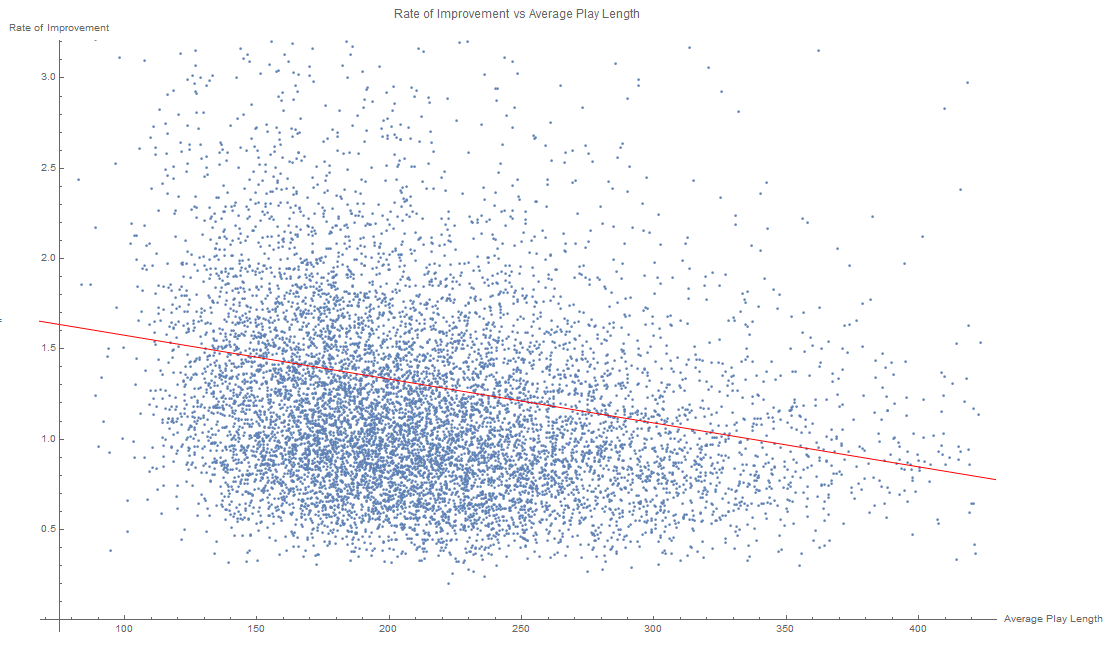
With a linear fit with r = -0.116515. This shows there is a very slight negative linear correlation between the average length of each play of the player, and the efficiency the player obtains pp.
One problem with defining the rate of improvement as pp/hitcount is that, as seen in the data, the expected amount of pp given a certain hitcount is not linear, but rather roughly a monotonically increasing quasi-convex function. This means that the pp/hitcount value tends to be higher when the player is higher ranked (which contradicts the hypothesis previously made that low-ranked players tend to show higher rates of pp/hitcount). The solution given by Railey2 is filtering to narrowed ranges of ranking (which works is the range is small enough to make the relationship between pp and hitcount roughly linear).
Instead, I define rate of improvement as the expected hitcount given the amount of pp of the player, divided by the hitcount of the player. E(hitcount|pp)/hitcount. This has the advantage of being dimensionless value that is invariant towards non-linear scaling transforms of the measurements of pp, the formula for rate of improvement can be applied to all ranges of pp rankings even if the relationship is not linear.
A problem is that it is dubious to consider obtaining pp the same as improving at the game. I'd rather call the variable "pp farming efficiency" instead of "rate of improvement".
For finding the expected hitcount given the amount of pp, I did an isotonic regression of the data, which is a non-parametric fit that only assumes that the relationship between the variables is non-decreasing.
Using that fitted curve to calculate rates of improvement, we obtain this graph:
With a linear fit with r = -0.116515. This shows there is a very slight negative linear correlation between the average length of each play of the player, and the efficiency the player obtains pp.
Full Tablet wrote:
With a linear fit with r = -0.116515. This shows there is a very slight negative linear correlation between the average length of each play of the player, and the efficiency the player obtains pp.
No offence but you must be crazy to call that a correlation.
Technically it's a correlation, albeit an awful one that certainly doesnt show any significant relation between the two things. To conclude something meaningful from it would be quite an extrapolation.
Almost wrote:
Full Tablet wrote:
With a linear fit with r = -0.116515. This shows there is a very slight negative linear correlation between the average length of each play of the player, and the efficiency the player obtains pp.
No offence but you must be crazy to call that a correlation.
Considering the large sample size (n=10000) and r = -0.116515, then the variables are significantly correlated (i.e. the null hypothesis of the variables having no correlation whatsoever is rejected) at a significance level of 1%.
Example of variables not significantly correlated
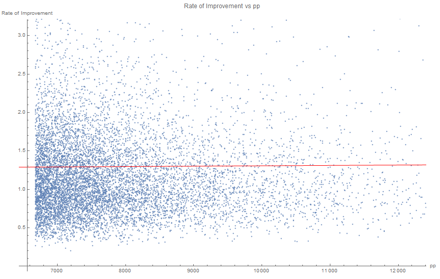
With r=0.0054, which is not a significant correlation (which is not surprising, since the "rate of improvement" was defined in a way that makes it uncorrelated with pp)
With r=0.0054, which is not a significant correlation (which is not surprising, since the "rate of improvement" was defined in a way that makes it uncorrelated with pp)
Full Tablet wrote:
Almost wrote:
Full Tablet wrote:
With a linear fit with r = -0.116515. This shows there is a very slight negative linear correlation between the average length of each play of the player, and the efficiency the player obtains pp.
No offence but you must be crazy to call that a correlation.
Considering the large sample size (n=10000) and r = -0.116515, then the variables are significantly correlated (i.e. the null hypothesis of the variables having no correlation whatsoever is rejected) at a significance level of 1%.
Example of variables not significantly correlated
With r=0.0054, which is not a significant correlation (which is not surprising, since the "rate of improvement" was defined in a way that makes it uncorrelated with pp)
The correlation is so poor that if you picked a random player with a certain average play length, you would literally have no idea what their rate of improvement would be because there's so much noise in the data. It really doesn't matter how much data you have, this data doesn't show anything meaningful.
Almost wrote:
The correlation is so poor that if you picked a random player with a certain average play length, you would literally have no idea what their rate of improvement would be because there's so much noise in the data. It really doesn't matter how much data you have, this data doesn't show anything meaningful.
https://en.wikipedia.org/wiki/Law_of_large_numbers
https://en.wikipedia.org/wiki/Insensitivity_to_sample_size
https://en.wikipedia.org/wiki/Correlation_does_not_imply_causation
Given the data, we can conclude with confidence that there is indeed a negative correlation between the variables in the population (high-ranked osu! players), and that the correlation between them is not coincidental, even though, as you said, for each specific player we can't predict accurately their improvement rate given the average length of their plays.
Now, for concluding there is a causation (having low average play length increases the efficiency of obtaining pp), there are still other things to consider and to prove:
- Prove That the relationship can not be explained by a third factor, that both decreases the average play length, and increases the improvement rate (or vice-versa).
- Prove that being efficient at obtaining pp doesn't somehow decrease the average play length. (This proof is sufficient, but not necessary, since there is also the possibility of bidirectional causation).
- In the case of generalizing to a bigger population (for example, all osu! players, instead of just high-ranked osu! players), one would need to prove there isn't something inherently different between the two groups (high-ranked and lower-ranked) that affects the correlation or causation. For this, it would be useful to repeat the analysis but with a random sample of all players instead of only taking the top 10k.
- In the case of trying to prove that retrying mid-play is beneficial for obtaining pp, one would need to account for differences between lengths in different maps played by different players. As far as we know, it is also possible that players that play longer maps tend to get pp less efficiently, regardless if they retry or not.
Full Tablet wrote:
Almost wrote:
The correlation is so poor that if you picked a random player with a certain average play length, you would literally have no idea what their rate of improvement would be because there's so much noise in the data. It really doesn't matter how much data you have, this data doesn't show anything meaningful.
https://en.wikipedia.org/wiki/Law_of_large_numbers
https://en.wikipedia.org/wiki/Insensitivity_to_sample_size
https://en.wikipedia.org/wiki/Correlation_does_not_imply_causation
Given the data, we can conclude with confidence that there is indeed a negative correlation between the variables in the population (high-ranked osu! players), and that the correlation between them is not coincidental, even though, as you said, for each specific player we can't predict accurately their improvement rate given the average length of their plays.
Now, for concluding there is a causation (having low average play length increases the efficiency of obtaining pp), there are still other things to consider and to prove:
- Prove That the relationship can not be explained by a third factor, that both decreases the average play length, and increases the improvement rate (or vice-versa).
- Prove that being efficient at obtaining pp doesn't somehow decrease the average play length. (This proof is sufficient, but not necessary, since there is also the possibility of bidirectional causation).
- In the case of generalizing to a bigger population (for example, all osu! players, instead of just high-ranked osu! players), one would need to prove there isn't something inherently different between the two groups (high-ranked and lower-ranked) that affects the correlation or causation. For this, it would be useful to repeat the analysis but with a random sample of all players instead of only taking the top 10k.
- In the case of trying to prove that retrying mid-play is beneficial for obtaining pp, one would need to account for differences between lengths in different maps played by different players. As far as we know, it is also possible that players that play longer maps tend to get pp less efficiently, regardless if they retry or not.
Just to state it out here, I have not accused you of implying causation. I am simply pointing out that there really is no correlation here at all. To put it simply, you are extrapolating noise! You can't just look at the r number and then say there is or is not correlation. If you eyeball the data, it's plainly obvious that there's no correlation. The fact you need a computer to draw out a line for you is evidence of this.
I think we can all agree that there is no conclusion about skill to draw from pp, a flawed and constantly exploited skill metric (if it even counts as one).
Almost wrote:
Just to state it out here, I have not accused you of implying causation. I am simply pointing out that there really is no correlation here at all. To put it simply, you are extrapolating noise! You can't just look at the r number and then say there is or is not correlation. If you eyeball the data, it's plainly obvious that there's no correlation. The fact you need a computer to draw out a line for you is evidence of this.
If the data were totally uncorrelated, then the probability of obtaining a value of r=-0.116515 or less, with a sample size of n=10000, would be very low (less than 0.001%). The null hypothesis of there being no correlation in the population is rejected. This doesn't mean that the correlation is strong (in fact, it is very weak), it just means that the correlation exists.
You are probably thinking about the possibility of there being measurement errors in the variables by noise. If the measurement noise in the samples is big enough and correlated, this can lead to finding spurious correlations that do not represent the true trends in the population.
Possible sources of measurement errors in the data are:
- Cheaters, who aren't representative of the population we are interested in. Cheating leads to a fake higher improvement rate over not cheating, but it is reasonable to assume that it also leads to a higher average play length (due to not needing to retry beatmaps to get good scores). Thus, cheaters actually make the apparent negative correlation weaker than the real correlation.
- People who selectively only submit plays that give them pp, giving them a fake low hitcount and playcount value, and thus a fake high improvement rate. Similar to the previous case, this also leads to higher average play length due to retries not being counted in the data.
- People who play offline, or play unranked beatmaps. Similar to the previous case, this behavior also gives a fake high improvement rate (but not as much as the previous case), but there shouldn't be a correlation with average play length (or, maybe, there is a positive correlation, since playing unranked/offline might be correlated with not caring about obtaining pp, and that attitude is in turn correlated with retrying less or playing longer maps).
- People who multi-account, or that have had scores deleted. This leads to a higher measured improvement rate, but shouldn't affect the average play length.
- Plays that have been randomly lost due to connection problems. This causes uncorrelated and random noise in the measurements.
- Other sources of noise I haven't thought of.
Considering the sources of noise I mentioned, it is actually reasonable to assume that the real correlation is stronger than the measured correlation, unless I am missing some important source of measurement errors, or I am assuming wrong about the correlations in the sources of noise.
Full Tablet wrote:
If the data were totally uncorrelated, then the probability of obtaining a value of r=-0.116515 or less, with a sample size of n=10000, would be very low (less than 0.001%). The null hypothesis of there being no correlation in the population is rejected. This doesn't mean that the correlation is strong (in fact, it is very weak), it just means that the correlation exists.
You are probably thinking about the possibility of there being measurement errors in the variables by noise. If the measurement noise in the samples is big enough and correlated, this can lead to finding spurious correlations that do not represent the true trends in the population.
Possible sources of measurement errors in the data are:
- Cheaters, who aren't representative of the population we are interested in. Cheating leads to a fake higher improvement rate over not cheating, but it is reasonable to assume that it also leads to a higher average play length (due to not needing to retry beatmaps to get good scores). Thus, cheaters actually make the apparent negative correlation weaker than the real correlation.
- People who selectively only submit plays that give them pp, giving them a fake low hitcount and playcount value, and thus a fake high improvement rate. Similar to the previous case, this also leads to higher average play length due to retries not being counted in the data.
- People who play offline, or play unranked beatmaps. Similar to the previous case, this behavior also gives a fake high improvement rate (but not as much as the previous case), but there shouldn't be a correlation with average play length (or, maybe, there is a positive correlation, since playing unranked/offline might be correlated with not caring about obtaining pp, and that attitude is in turn correlated with retrying less or playing longer maps).
- People who multi-account, or that have had scores deleted. This leads to a higher measured improvement rate, but shouldn't affect the average play length.
- Plays that have been randomly lost due to connection problems. This causes uncorrelated and random noise in the measurements.
- Other sources of noise I haven't thought of.
Considering the sources of noise I mentioned, it is actually reasonable to assume that the real correlation is stronger than the measured correlation, unless I am missing some important source of measurement errors, or I am assuming wrong about the correlations in the sources of noise.
The probability of such a correlation occurring is completely irrelevant. You could get 2 random data sets that happen to spuriously correlate and find they have a 0.001% of not being correlated statistically. Therefore, moot point.
I also find engaging in hypothesizing what the 'true' correlation to be rather pointless as it's realistically impossible to gain this data. Yes, you could potentially find a real negative correlation but at the same time, you could find the opposite to be true. This analysis provides really nothing meaningful and nobody should really be wasting their time thinking too much about it.
Antiforte wrote:
I think we can all agree that there is no conclusion about skill to draw from pp, a flawed and constantly exploited skill metric (if it even counts as one).
There is no such thing as a perfect skill measuring system. It's impossible to satisfy everyone. Is pp flawed and exploited? Yes but any system you cook up will be the same. I still think pp is somewhat relevant since it guides the skill acquiring habits of the majority of the community.
Almost wrote:
The probability of such a correlation occurring is completely irrelevant. You could get 2 random data sets that happen to spuriously correlate and find they have a 0.001% of not being correlated statistically. Therefore, moot point.
I also find engaging in hypothesizing what the 'true' correlation to be rather pointless as it's realistically impossible to gain this data. Yes, you could potentially find a real negative correlation but at the same time, you could find the opposite to be true. This analysis provides really nothing meaningful and nobody should really be wasting their time thinking too much about it.
https://en.wikipedia.org/wiki/Statistical_significance
https://en.wikipedia.org/wiki/Effect_size
https://en.wikipedia.org/wiki/Misuse_of_p-values
If you measure in a sample that there is a negative correlation, and the probability of not measuring that there is a negative correlation in case there is no negative correlation is 99.999%, the most reasonable conclusion is that there is indeed a negative correlation. If you only accepted empirical conclusions that have 100% certainty, you wouldn't be able to conclude anything, you wouldn't even conclude that gravity exists or that the Sun shines.
You are confusing statistical significance with effect size or magnitude of the effect. An example of high statistical significance with low effect size: a statistical study finds, with high confidence, that, obese people, eating a certain plant at least weekly, lose 0.1±2.0 more kilograms of weight each month (compared to not eating the plant at least weekly).
While the results might appear to be worthless (after all, the average effect is so small, and the variance of the outcome is so high, it is not worth it to influence the variable hoping to change the outcome), it does tell us some important things.
First of all, it tells us that it is not reasonable to expect the opposite effect of what was seen (that increasing the average play length increases the efficiency of getting pp). Also, the low value of of r tells us that, while in average we should expect a negative effect in pp farming efficiency when increasing the average play length, we can't predict the precise outcome with confidence.
Full Tablet wrote:
https://en.wikipedia.org/wiki/Statistical_significance
https://en.wikipedia.org/wiki/Effect_size
https://en.wikipedia.org/wiki/Misuse_of_p-values
If you measure in a sample that there is a negative correlation, and the probability of not measuring that there is a negative correlation in case there is no negative correlation is 99.999%, the most reasonable conclusion is that there is indeed a negative correlation. If you only accepted empirical conclusions that have 100% certainty, you wouldn't be able to conclude anything, you wouldn't even conclude that gravity exists or that the Sun shines.
You are confusing statistical significance with effect size or magnitude of the effect. An example of high statistical significance with low effect size: a statistical study finds, with high confidence, that, obese people, eating a certain plant at least weekly, lose 0.1±2.0 more kilograms of weight each month (compared to not eating the plant at least weekly).
While the results might appear to be worthless (after all, the average effect is so small, and the variance of the outcome is so high, it is not worth it to influence the variable hoping to change the outcome), it does tell us some important things.
First of all, it tells us that it is not reasonable to expect the opposite effect of what was seen (that increasing the average play length increases the efficiency of getting pp). Also, the low value of of r tells us that, while in average we should expect a negative effect in pp farming efficiency when increasing the average play length, we can't predict the precise outcome with confidence.
If anything, you're the one confusing the value of the p value. Firstly, you can use a simple p value correlation calculator (like this one) and find that you only really need the r value as well as the number of samples to calculate the p value. Therefore, what dictates the p value is simply the number of samples; with a r score further away from 0 requiring a higher number of samples to give a lower p value.
Again, you cannot simply just look at the numbers only as the numbers only tell you half the story. If you were to just look at the numbers alone, it's evident that a correlation exists. However, intuitively looking at the data itself, it is clearly evident that a real correlation does not exist for practical purposes.
Also, any conclusions you might draw from this data will be seriously flawed due to all the possible sources of measurement errors in the data that you mentioned earlier. This means that drawing any conclusions at all is quite dangerous.
Almost wrote:
If anything, you're the one confusing the value of the p value. Firstly, you can use a simple p value correlation calculator (like this one) and find that you only really need the r value as well as the number of samples to calculate the p value. Therefore, what dictates the p value is simply the number of samples; with a r score further away from 0 requiring a higher number of samples to give a lower p value.
Again, you cannot simply just look at the numbers only as the numbers only tell you half the story. If you were to just look at the numbers alone, it's evident that a correlation exists. However, intuitively looking at the data itself, it is clearly evident that a real correlation does not exist for practical purposes.
Also, any conclusions you might draw from this data will be seriously flawed due to all the possible sources of measurement errors in the data that you mentioned earlier. This means that drawing any conclusions at all is quite dangerous.
A r score further away from 0 requires a lower amount of samples to obtain a certain p value, not a higher amount of samples.
Looking at the scatter plot is more useful when the sample is smaller. Intuition generally fails when the amount of data is more than what one can visually process. In particular, by looking at the graph, we can correctly infer that the correlation is not high, but that doesn't imply that the conclusions you draw from the data aren't relevant. The correlation is not to be ignored if the underlying implications of such a weak correlation make sense to be reported to a research community. Any r > 0.1 on a large data set is always something to look into.
The attitude of rejecting conclusions because they aren't visually intuitive can and does lead people to prefer smaller sample sizes over bigger sample sizes for drawing conclusions from, which is clearly a mistake.
https://en.wikipedia.org/wiki/Correction_for_attenuation
As I said earlier, if we consider the sources of the error, it is actually more likely that the real correlation is higher than what was found in the analysis, than the other way around. It takes particular kinds of measurement errors to cause spurious correlations.
Full Tablet wrote:
A r score further away from 0 requires a lower amount of samples to obtain a certain p value, not a higher amount of samples.
Whoops, yes my bad here.
Full Tablet wrote:
Looking at the scatter plot is more useful when the sample is smaller. Intuition generally fails when the amount of data is more than what one can visually process. In particular, by looking at the graph, we can correctly infer that the correlation is not high, but that doesn't imply that the conclusions you draw from the data aren't relevant. The correlation is not to be ignored if the underlying implications of such a weak correlation make sense to be reported to a research community. Any r > 0.1 on a large data set is always something to look into.
https://en.wikipedia.org/wiki/Correction_for_attenuation
As I said earlier, if we consider the sources of the error, it is actually more likely that the real correlation is higher than what was found in the analysis, than the other way around. It takes particular kinds of measurement errors to cause spurious correlations.
Compare the plot you provided with these 3 plots.
Visually you can see it's more similar to the 3rd no correlation plot than to either of the positive or negative correlation plots.
Again, just because you can mathematically calculate an r value greater than or less than 0.1 with a significant p value doesn't mean it's 'real' correlation at all. Again, the p value is predicated more on the sample size than anything else so as long as you have enough samples you can get a significant p value no matter how erroneous everything else is. Anyway, a correlation of -0.11 is already a super weak correlation and paired up with the fact that the data has an enormous amount of variance as well as the poor quality of data allows us to conclude that nothing of meaning can really be drawn from this analysis.
Now to explain what we see further, you can see that the vast bulk of the play lengths of the players in the data set tend to be around the 150-250 range with far fewer players on the higher end compared to the lower end of the range. Also, the rate of improvement is also more clumped towards the lower end of the range (around 0.5-1.5) no matter what average play length you pick. The line of best fit in the plot you gave would clearly skew more towards the negative side of things due to the higher representation of the variance in the lower average play length side of the plot. You can't really extrapolate that this correlation would hold if you were to have more players in the data set on the higher end of the average play length range as the variance is so huge on all ends of the spectrum which would likely end up just leading to a no correlation result.
Almost wrote:
Compare the plot you provided with these 3 plots.
Visually you can see it's more similar to the 3rd no correlation plot than to either of the positive or negative correlation plots.
Yes, it is true that the data is closer to no correlation than perfect correlation.
Almost wrote:
Again, just because you can mathematically calculate an r value greater than or less than 0.1 with a significant p value doesn't mean it's 'real' correlation at all. Again, the p value is predicated more on the sample size than anything else so as long as you have enough samples you can get a significant p value no matter how erroneous everything else is. Anyway, a correlation of -0.11 is already a super weak correlation and paired up with the fact that the data has an enormous amount of variance as well as the poor quality of data allows us to conclude that nothing of meaning can really be drawn from this analysis.
If there is no correlation, it is almost impossible to obtain a value of r<=-0.11 with a large sample. When there is no correlation, as you increase the sample size, |r| tends to approach 0, so it is not true that as you increase the sample size you are more likely to find a statistically significant correlations when there are actually none.
Almost wrote:
Now to explain what we see further, you can see that the vast bulk of the play lengths of the players in the data set tend to be around the 150-250 range with far fewer players on the higher end compared to the lower end of the range. Also, the rate of improvement is also more clumped towards the lower end of the range (around 0.5-1.5) no matter what average play length you pick. [...] You can't really extrapolate that this correlation would hold if you were to have more players in the data set on the higher end of the average play length range as the variance is so huge on all ends of the spectrum which would likely end up just leading to a no correlation result.
Yes, due to not having much data outside the 100-250 play-length, we can't infer much about the effect of play length on improvement rate outside that play-length range (but still, we do have information about the effect inside the range).
If we sampled again with more data outside that range, and found that the correlation is weaker across all the range, then we would need to check for non-linear relationships between the variables. For example, it is possible that there is a bitter spot in play-length (for small play-lengths, increases of play-length tends to decrease improvement rate, and for big play-lengths, increases of play-length tends to increase improvement rate).
Almost wrote:
The line of best fit in the plot you gave would clearly skew more towards the negative side of things due to the higher representation of the variance in the lower average play length side of the plot.
I am not sure I understand what you are trying to say here.
Full Tablet wrote:
If there is no correlation, it is almost impossible to obtain a value of r<=-0.11 with a large sample. When there is no correlation, as you increase the sample size, |r| tends to approach 0, so it is not true that as you increase the sample size you are more likely to find a statistically significant correlations when there are actually none.
As I said mathematically, yes there is a correlation but the issue is whether such a correlation is practically relevant. The amount of variance in the plot says no. Essentially, this correlation is purely fit to noise.
Full Tablet wrote:
Yes, due to not having much data outside the 100-250 play-length, we can't infer much about the effect of play length on improvement rate outside that play-length range (but still, we do have information about the effect inside the range).
And you're just going to infer that the correlation is the same?? Not that it matters though since there's just way too much variance in the data.
Full Tablet wrote:
If we sampled again with more data outside that range, and found that the correlation is weaker across all the range, then we would need to check for non-linear relationships between the variables. For example, it is possible that there is a bitter spot in play-length (for small play-lengths, increases of play-length tends to decrease improvement rate, and for big play-lengths, increases of play-length tends to increase improvement rate).
Again, there's really no point in pontifiyng things outside the realm of possibility. It's realistically impossible to gather this data that's actually very clean.
Full Tablet wrote:
I am not sure I understand what you are trying to say here.
Correlation coefficient calculation is based off the least squares method which basically finds the line of best fit for a given set of data points. Since the distribution of this data is skewed towards the lower improvement ranges for basically all play lengths and there also being lack of data for the higher play lengths, there is a lower representation of the higher rates of improvement in the high play lengths. Simply put, since the distribution of the data is like below, if you were to have more data for the higher play lengths, you'd likely just get a uniform plot without any real change in the rate of improvement vs average play length since the distribution is pretty linear no matter the play length.
Railey would rejoice if he knew that his drama bait thread is thriving once again.
Full Tablet, can you post density scatter plots with contours for the results?
Almost wrote:
Full Tablet wrote:
If there is no correlation, it is almost impossible to obtain a value of r<=-0.11 with a large sample. When there is no correlation, as you increase the sample size, |r| tends to approach 0, so it is not true that as you increase the sample size you are more likely to find a statistically significant correlations when there are actually none.
As I said mathematically, yes there is a correlation but the issue is whether such a correlation is practically relevant. The amount of variance in the plot says no. Essentially, this correlation is purely fit to noise.
You are just repeating your points here. As I said earlier, there are conclusions that are practically relevant even if the correlation found is weak. For example, we can conclude that the correlation is not null nor positive (so it is not reasonable to increase your average playcount expecting to get pp more efficiently, and "never retry" is likely bad advice if one seeks to gain pp efficiently), we can also conclude that the correlation is weak, so we can't confidently predict the outcome based on the variables (in other words, "Your mileage might vary").
You seem to be confusing measurement noise with inherent noise in the data; measurement noise does weaken some inferences you might make from the data (but not all inferences, such as the existence of correlation, except when the noise itself is correlated), inherent noise (noise we would obtain even if the measurements are perfect) does not make the inferences less reliable, it just makes predictions less reliable.
Almost wrote:
Full Tablet wrote:
Yes, due to not having much data outside the 100-250 play-length, we can't infer much about the effect of play length on improvement rate outside that play-length range (but still, we do have information about the effect inside the range).
And you're just going to infer that the correlation is the same?? Not that it matters though since there's just way too much variance in the data.
I am not inferring that the correlation is the same outside the points we have more data on. I am saying that we can't infer as confidently outside the range as we would do inside the range.
Almost wrote:
Full Tablet wrote:
If we sampled again with more data outside that range, and found that the correlation is weaker across all the range, then we would need to check for non-linear relationships between the variables. For example, it is possible that there is a bitter spot in play-length (for small play-lengths, increases of play-length tends to decrease improvement rate, and for big play-lengths, increases of play-length tends to increase improvement rate).
Again, there's really no point in pontifiyng things outside the realm of possibility. It's realistically impossible to gather this data that's actually very clean.
Acknowledging what we don't know is also important. If we aren't able to know about something, we should take into consideration all possibilities about it (which is not the same as assuming that one of the possibilities is true, which would be something obviously wrong to do).
Almost wrote:
Correlation coefficient calculation is based off the least squares method which basically finds the line of best fit for a given set of data points. Since the distribution of this data is skewed towards the lower improvement ranges for basically all play lengths and there also being lack of data for the higher play lengths, there is a lower representation of the higher rates of improvement in the high play lengths. Simply put, since the distribution of the data is like below, if you were to have more data for the higher play lengths, you'd likely just get a uniform plot without any real change in the rate of improvement vs average play length since the distribution is pretty linear no matter the play length.
Do you think that the sampling process was skewed towards selecting points that have low improvement ranges? The fact that the data obtained has a skewed distribution doesn't mean that the sample is biased, as far as we know, that skew seems to be a characteristic of the population.
Also, if the distribution of the independent variable in the data is skewed towards lower values, it is not true that you should expect getting a false negative slope in the linear regression of the data.
Example:
Suppose that in the population, there is an inherent randomness in the value obtained in the dependent variable for each point in the independent variable, with the randomness following a skewed distribution.
(The closer the point is to white, the more probable is to obtain that value). The best possible prediction of y given x is a linear function y(x) = 0.01x, and the true correlation between the two variables is r=0.115216.
Now, we do a sample that is very skewed towards taking points with low values of x:
This sample has a linear regression of y(x) = 0.0000122334 + 0.0100465x, and r=0.115216, which is pretty close to the ideal parameters. If we repeat this skewed sampling several times we obtain similar results. There is no tendency to find slopes when we shouldn't with the skewed sampling.
Another example:
Suppose that the population follows this distribution for each x:
Which has an ideal prediction function y(x)=0.01x^2, and r^2=0.258148. Attempting a linear regression with a sample of this population would fail with r very close to 0.
Now let's take a very skewed sample:
A linear regression gives y(x)=0.33314 -6.47732*10^-6 x, with r=-0.0000643552 (so it fails).
A quadratic regression gives y(x)=0.00303735 -6.47732*10^-6 x+0.00990298 x^2, with r^2=0.258148. So even a sample this skewed reproduces the non-linearity of the population.
Abraker wrote:
Full Tablet, can you post density scatter plots with contours for the results?
Here it is (using a Gaussian kernel).
I also included a high-degree (7) polynomial regression curve, which has r^2=0.0225744 (|r|=0.150248, better than the one in the linear model with r = -0.116515), which is significant at a significance level of 1%. This curve is better for predicting rate of improvement given the average hitcount in the white area of the graph (where we have the most information), but high-degree curves are worse at extrapolating compared to linear curves, and the low value of r^2 indicates that the predictions are still not reliable.
Doing a F-test to check whether or not the high-degree polynomial model fits the data significantly better than the linear model (null hypothesis: high-degree polynomial model does not provide a significantly better fit than the linear model), we conclude that the polynomial model is significantly better with a false-rejection probability less than 1%.
Full Tablet wrote:
You are just repeating your points here. As I said earlier, there are conclusions that are practically relevant even if the correlation found is weak. For example, we can conclude that the correlation is not null nor positive (so it is not reasonable to increase your average playcount expecting to get pp more efficiently, and "never retry" is likely bad advice if one seeks to gain pp efficiently), we can also conclude that the correlation is weak, so we can't confidently predict the outcome based on the variables (in other words, "Your mileage might vary").
You seem to be confusing measurement noise with inherent noise in the data; measurement noise does weaken some inferences you might make from the data (but not all inferences, such as the existence of correlation, except when the noise itself is correlated), inherent noise (noise we would obtain even if the measurements are perfect) does not make the inferences less reliable, it just makes predictions less reliable.
There is both which makes drawing conclusions from this data very difficult. We do not know the effects of the noise in the data either. Yes, you can hypothesize the effects of potential noise in the data but you still can't effectively conclude that the correlation will only get more negative unless you have data to prove it. For example, there might be a "critical mass" sort of effect whereby having an average play length above a certain cut off produces greater rates of improvement. Obviously, that's a bit of a stretch however, it's still in the realm of possibilities along with any other sort of wacky effects.
Full Tablet wrote:
Do you think that the sampling process was skewed towards selecting points that have low improvement ranges? The fact that the data obtained has a skewed distribution doesn't mean that the sample is biased, as far as we know, that skew seems to be a characteristic of the population.
Also, if the distribution of the independent variable in the data is skewed towards lower values, it is not true that you should expect getting a false negative slope in the linear regression of the data.
I'm fully aware of the fact that the skewed distribution is likely just a characteristic of the population. Your assumption is that the skew in the rate of improvement becomes more pronounced as you increase the play length but it's not possible to say this given the lack of data for the higher play lengths.
Ok, Full Tablet, I am more eager to say correlating the data you gathered is a mistake. It's like waving data saying "oh look correlations might mean something", but we can't use those correlations for anything useful. You are focusing on the wrong thing when you can be focusing on something that can actually be worthwhile.
There is useful information concerning the sample you gathered in probabilistic sense. So for example, picking a random player and knowing their PP allows us to determine the probability their hitcount is something. Or vice-versa, knowing their hitcount we can determine the probability their PP is something. Let me do the pp vs hitcount data for you.
Knowing the pp vs hitcount tendencies of the sample gathered, that can be used for something useful after classifying regions. Let's take the 4 corner extremes of the space, and just apply idealistic conditions to why we would find them there.
Looking at the density plot
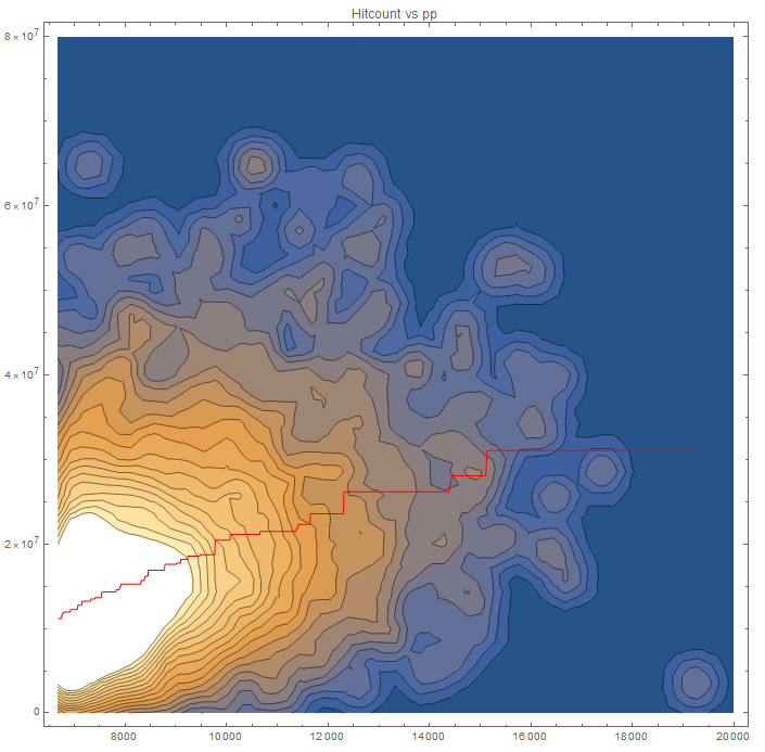
We can see that majority of the players are in the bottom left corner. Those are the players in the sample either don't play ranked or haven't played enough. We can call that the causal core. What's interesting to note is that casual core is not in the actual corner. Rather majority have some hitcount and pp. Further analysis of the casual core can reveal the expected average hitcount and pp of a casual player +/- some number due to variance.
There is is a relatively tiny % of players that appear in the the bottom right corner indicated they cheated or improved very fast. But thanks to the original scatter plot we know it's one point. If you know osu! history then it's obviously cookiezi. Still we shouldn't ignore the players on that lower edge, but I don't have an immediate answer to how that edge can be analyzed.
Finally we have this wide spread of players forming this outer shell. This resembles a sample of players that are arguably not casual, either having high hitcount or high pp or both.
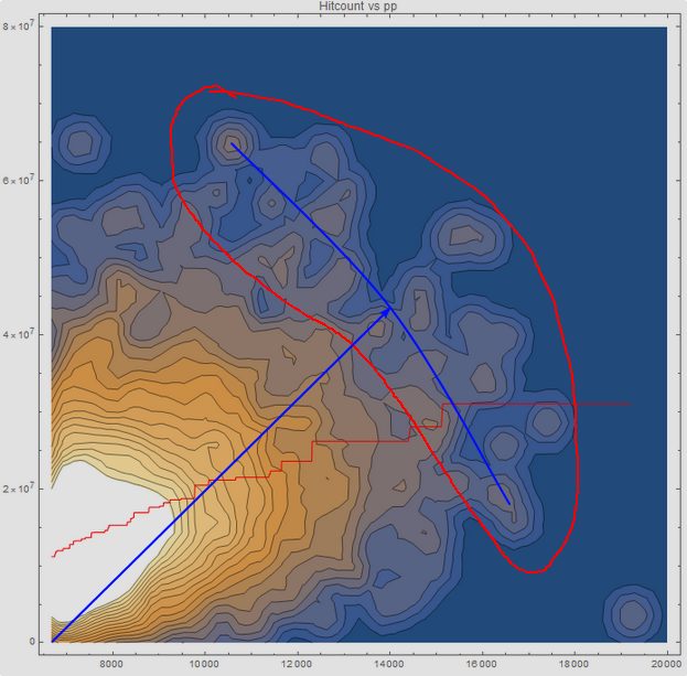
Isolating to just this region and analyzing can give additional info regarding that specific sample of players. I drew a vector and arc to give ideas of what can be analyzed, but I am blanking out on what that might be at the moment I am writing this. I'm not sure how much hitcount to pp would imply the player is having trouble gaining pp since the scale of hitcount to pp is kinda arbitrary.
All in all there are things in this data that can be looked into more deeply, but correlation like a linear regressions are not it.
---------
So to end this off let me classify all regions in shitpost like spirit
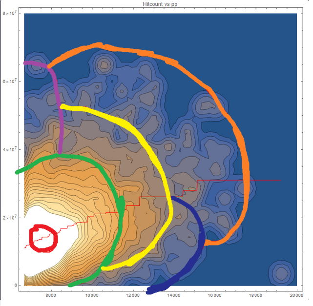
Some lines may need adjusting, but you get the point
There is useful information concerning the sample you gathered in probabilistic sense. So for example, picking a random player and knowing their PP allows us to determine the probability their hitcount is something. Or vice-versa, knowing their hitcount we can determine the probability their PP is something. Let me do the pp vs hitcount data for you.
Knowing the pp vs hitcount tendencies of the sample gathered, that can be used for something useful after classifying regions. Let's take the 4 corner extremes of the space, and just apply idealistic conditions to why we would find them there.
- Low hitcount, low pp - bottom left. This is a reasonable area to expect new players in or people that don't play ranked much.
Low hitcount, high pp - bottom right. This area indicates either extreme levels of improvement or cheating.
High hitcount, low pp - top left. This area includes players that would either have trouble improving, players playing to simply get into leaderboards, or just playing for the sake of playing.
High hitcount, high pp - top right. This area would display the effort of players that try hard to gain pp.
Looking at the density plot
We can see that majority of the players are in the bottom left corner. Those are the players in the sample either don't play ranked or haven't played enough. We can call that the causal core. What's interesting to note is that casual core is not in the actual corner. Rather majority have some hitcount and pp. Further analysis of the casual core can reveal the expected average hitcount and pp of a casual player +/- some number due to variance.
There is is a relatively tiny % of players that appear in the the bottom right corner indicated they cheated or improved very fast. But thanks to the original scatter plot we know it's one point. If you know osu! history then it's obviously cookiezi. Still we shouldn't ignore the players on that lower edge, but I don't have an immediate answer to how that edge can be analyzed.
Finally we have this wide spread of players forming this outer shell. This resembles a sample of players that are arguably not casual, either having high hitcount or high pp or both.
Isolating to just this region and analyzing can give additional info regarding that specific sample of players. I drew a vector and arc to give ideas of what can be analyzed, but I am blanking out on what that might be at the moment I am writing this. I'm not sure how much hitcount to pp would imply the player is having trouble gaining pp since the scale of hitcount to pp is kinda arbitrary.
All in all there are things in this data that can be looked into more deeply, but correlation like a linear regressions are not it.
---------
So to end this off let me classify all regions in shitpost like spirit
- Red - Causal core
Green - Skrubs
Yellow - Mediocres
Orange - Poggers
Purple - Accers
Dark Blue - Cheaters
Some lines may need adjusting, but you get the point
Isn't it as simple as
stream players have big hitcount/playcount, and they get pp slower
and jump players have low hitcount/playcount, and they get pp faster? But not necessarily bcs of retries, but bcs they're playing farm maps
The hitcount/playcount = average play length is only true if everyone plays the same maps. And of course if you have huge hitcount/playcount you're not playing short farm maps