How does PP actually work out? Dissecting the PP algorithm of osu!
Alternative full text in my blog: https://turou.fun/osu/pp-system-en/
In this paper, we mainly investigate the PP algorithm in osu! standard ruleset, aiming to help other players who are interested in the PP algorithm to quickly build up their knowledge of the algorithm.
As most of the content is the author's personal understanding and experience, there may be errors or bias, readers are welcome to propose recommendations
The code snippets in this article are derived from rosu-pp, a Rust performance implementation of osu!lazer, which is currently the most popular library for performance calculation.
In addition, the article is intended for readers with minimal programming experience, who do not need in-depth knowledge of Rust.
A first look
Two-step calculation
Instead of complex algorithms, let's talk about the surface first. Simply speaking, the PP system evaluates the concepts of difficulty of the beatmap and how well player plays.
There is a widespread misconception that the PP system evaluates these concepts based on replay, which is a false perception. In fact, the calculation is a two-step process.
The first step is to calculate the Beatmap Difficulty (which is usually based on all the objects in beatmap)
The second step is to calculate the final PP value based on the Beatmap Difficulty calculated in the first step and a number of other player variables (e.g., Player Acc, Miss count, Max Combo).
As you can imagine, the first step of the calculation takes into account the base value of the interaction between the objects, while the second step of the calculation is to adjust the multiplier according to the performance of the players on the base value. Let's take a simple example:
Cookiezi scored 939PP in FDFD, while mrekk scored 926PP and Accolibed scored 640PP. All three of them have the same base value in the first step of the calculation, but different factors in the second step. Cookiezi hit more accurate than mrekk, and got a higher acc bonus. Accolibed dropped a miss, and got a miss penalize. In the end, all sorts of bonuses and penalizes were applied to the base value, and then, final value was calculated.
For this reason, it is much more efficient to group the scores by beatmap first when calculating a large number of scores. since the first calculation (which is also the decisive speed step) is only performed once.
Difficulty & Skills
After the above exploration, we understand that the calculation of Difficulty is the most important thing, which is the key to tell the difference among beatmaps
The designers of osu! intentionally evaluated difficulty in multiple dimensions, and the concept of Skill was clarified over many years of iteration.
As you know, osu! standard should include at least two skills, Aim and Speed, and of course, they do, as shown in the table below.
Since I don't know much about other modes, we will focus on osu!standard.
Skill & Calculus?
I'm sure you're already very interested in the specific calculations of Aim, Speed, but before we get started, let's have a look at how Skill is formed.
Imagine a score that is a few minutes long, how should we calculate its difficulty? This is actually a difficult question, and it is hard to measure difficulty since objects stacked on a time axis are just arrays of positions.
Readers who have taken calculus may be familiar with this example: a smooth surface may be irregular and it is difficult to calculate the area, but if the surface is subdivided infinitely and the smallest unit is considered to be a square, the problem is easily solved. That is, the whole surface is difficult to solve, but a slice is often easy to solve.
Skill calculation followed a similar process of differentiation followed by integration, in which objects are divided and treated separately.
Simply speaking, each hitobject can be considered as an atom that represents the difficulty, which is called strain in PP system. The final skill value (e.g. raw_aim, raw_speed) is actually the result of integrating (somehow adding up) the strains.
In osu! standard, most of the patterns (e.g. acute jumps, obtuse jumps) are Strain specific, i.e. we separate these patterns in the process of calculating one specific Strain. In the actual calculation, we can get many variables (such as the following) to assist us in determining the "difficulty of the current object".
We will approach these concepts in a step-by-step process in the following tutorials. Of course, in a bottom-up manner, we will focus on analyzing the process of Strain calculations.
Next, we will explore Aim & Speed Skills and try to find out how a single Strain is calculated.
Explore Aim
In rosu-pp, we can find skill definitions and implementations in the /osu/difficulty/skills folder.
Now let's try to start reading the source code of aim.rs.
In the above explanation, we have clarified the concept of objects are divided and treated separately. So obviously,
osu_curr_obj
Obviously, when the object is a spinner, the method returns 0.0 and does not perform any subsequent calculations.
Distance/Time=Speed
Here we will explain some terms, in order to better understand parameters.
strain_time
Indicates the time interval between the current object and the previous object, in milliseconds.
Calculated as:
It can also be calculated in the following way:
For most of the beatmap:
Normalized distance between the current object and the previous object, in osu!pixel
Calculated as:
Indicates the sliding distance of the slider object.
travel_time
Indicates the sliding time of the slider object.
min_jump_time
Indicates the time interval between the current object and the previous slider header after subtracting the sliding time.
Usually used if the previous object is a slider, if the previous object is not a slider, the value is equal to the strain_time.
min_jump_dist
Indicates the distance between the current object and the previous slider end after subtracting the sliding distance.
Usually used if the previous object is a slider, if the previous object is not a slider, this value is equal to lazy_jump_dist.
Now let's return to the code analysis part. I believe the most attractive part is the extend velocity, we will draw a graph to explain it
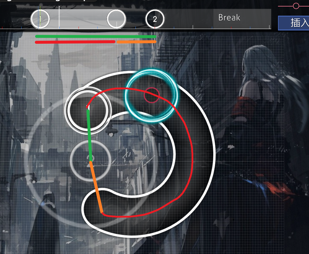
Now please consider Circle 2 as the current object, obviously, the green part is the
Since the previous object is a slider, the condition is met, and the velocities of the red part and the orange part are then calculated and summed to maximize with the original
Obviously, for this pattern, the sum of the velocities of the red part and the orange part is larger than that of the green part, so the subsequent value is used as the
Objectively speaking, extend velocity is a better representation of the speed of Slider 1 -> Circle 2.
Acute wide angle pattern
In the previous section, we calculated the base value of the strain based on the velocities, and in this section, the algorithm considers the typical acute and obtuse patterning to derive specific bonus.
Note: The code here has been trimmed, reordered and extracted to improve readability without changing the logic.
Here we divide the code into four parts according to the annotations: Rhythm Judgment, Base Calculation, Acute Bonus Calculation, and Repeat Penalty.
The rhythm is determined at the top level, so that only objects that meet the criteria will receive the extra bonuses.
First of all, the algorithm ensures that the rhythm change is small, limiting the time change between the current object and the previous object is within 25%.
Objectively speaking, a pattern can only be formed if the rhythm change is small. If the rhythm varies too much, it can't be called as pattern.
Base Calculation
Using GeoGebra, we can draw the following graphs, with the red line representing the wide-angle curve and the blue line representing the acute-angle curve.
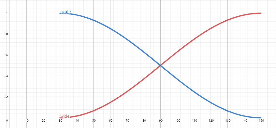
Above 30 degrees, the wide angle bonus grows smoothly with the angle. Below 150 degrees, the acute-angle bonus grows smoothly with the angle. Objectively, this is a natural design
First of all,
This is an interesting and logical conclusion. Needless to say, it's hard to jump at 300 BPM or more. Stream over 150 BPM may seem like an easy bonus, but consider this, streams less than 90 degrees require STRONG aim control abilities.
As mentioned in the comments, the algorithm only wants to consider wiggly acute angles, which can be understood as several consecutive objects matching the characteristics of acute angle pattern.
While casual and sudden acute is not included in the bonus range, which is reasonable, because it should not be considered as any pattern.
Then, the algorithm scales velocity, strain_time, and distance:
The bonus range of base1: 150 ~ 200 BPM stream (1/4 snapping)
The bonus range of base2: 50 ~ 100 units (center of one circle lies on the circumference of another circle ~ tangent circle)
Repeat Penalty
Here the repeated wide angle can be penalized by comparing the last bonus.
If last angle is sharper, the penalty factor f(x) will be reduced, thus imposing a lighter penalty on the repeated wide angle
The
Velocity Change
In the previous section, the algorithm applied bonus to the acute and wide angle patterns, based on the assumption that the velocities are similar, i.e., the velocity changes are within 25%.
In the following we will introduce the velocity change bonus, which has the opposite assumption from above, i.e., the velocity must be different, and we will analyze it using a similar procedure as in the previous section.
Here we divide the code into three parts: Ratio Calculation, Base Calculation, and Rhythm Change Penalty.
Based on
First, the
Next,
The intensity of the velocity change as a ratio of the speed bonus, couldn't be more appropriate!
Obviously, velocity change is used directly as the base value.
The limit ensures that only velocity changes within a certain range are considered when calculating velocity changes. This makes the bonus value focus more on velocity changes between closer objects and ignore changes between more distant objects.
Rhythm Change Penalty
The time-change penalty here uses a similar normalization technique. The value of bonus_base (which is actually interpreted as penalize_base) is in the range [0, 1].
We plot the image of bonus_base, where the x and y axes are the strain_time, and the z axis is the value of bonus_base:
It is clear that when the strain_time is constant, there is almost no penalty (the value of bonus_base is 1).
When there is a change in strain_time, we assume a horizontal and vertical coordinate, there is always a smaller bonus_base corresponding to it. The larger the change in time, the larger the penalty is.
We'll consider Circle 3 to be the current object, and Circle 2 to be the previous object, algorithm will use the velocities of both to calculate the penalty of Circle 3.
The speed of Circle 3 is calculated using the green line, which is a small distance and a long time, so the speed must be very small.
The speed of Circle 2 is calculated using the red line, which is a short time with a large distance, and the speed must be very large.
Without introducing a time-change penalty, the algorithm will consider Circle 3 to be more difficult because of the large velocity change that occurs.
But in fact, in the gameplay, because there is a long time interval between Circle 3 and the previous object, the speed change is no longer felt, and the difficulty of Circle 3 is pretty low at this time.
On the other hand, if we drag the timeline of 1, 2, 3, 4 evenly, then this is a difficult pattern, and the player needs some aim control when hitting Circle 3.
Base *= Bonus
The first thing we see in the code are some defined constants (in all caps and underlined), which specify the proportion of each bonus in the final calculation.These constants reflect the weights of the parameters involved in the final calculation
Besides the constants, there are a couple of calculations, the first being the slider bonus calculation, which is rather simple:
This type of slider bonus will mainly be applied to beatmaps with long, high speed sliders (like Genryuu Kaiko).
Also, the way
As we mentioned above, the conditions for applying acute bonus are very tough (300 BPM jumps, 150 BPM streams), which means that most of the objects will not get the acute bonus.
Looking at the values of the constants, we see that the multiplier for acute bonus is larger than the multiplier for wide bonus, which provides higher rewards for more difficult and demanding patterns.
Simply speaking, most of the object bonus comes from the Wide Angle + Speed formula, and those common beatmaps don't even have a chance to get any Acute Angle bonus.
Explore Speed
Similar to Aim, let's first focus on the ISkill implementation of Speed in speed.rs, focusing on the
The Rhythm Complexity (RhythmEvaluator) here is the concept introduced in November 2021 Rework by Xexxar.
The Rework was controversial and highly publicized, yet it somewhat prevented Aim from becoming the main way to get PP, and brought osu! back from being a gopher simulator. We'll focus on that part later.
SpeedEvaluator
Before we start introducing SpeedEvaluator, let's expand on some concepts:
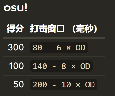
The hit window (in ms) can be seen in-game by hovering the cursor over the 3D position of the beatmap in the upper-left corner. osu!standard mode calculates it like this.
Algorithms always need to be iteratively updated to follow the mapper's talent, and innovative beatmaps can often push PP systems to update, this is how doubletapness was introduced
The introduction of doubletapness comes from the beatmap below:

It should be noticeable that there are several single beats in the segment that require double-tapping, which, in Speed calculations, is judged to be an extremely high-speed cut, and what's more, this will be exacerbated by the DTHR.
The
The
apollo-dw's name will also appear below.
Velocity & Distance
The intent of limiting
It takes into account whether the time between objects is less than 300 hit window, and if it is less, it will nerf the strain_time.
Here we have graphed
The calculation of dist is very similar to the concept of velocity extends in Aim, so let's reintroduce the image here:
Please consider Circle 2 as the current object, the dist of Circle 2 is the sum of the red and orange distances.
RhythmEvaluator
Since RhythmEvaluator is quite complex, we will first explain the theory in general and then analyze it with the code.
First of all, the RhythmEvaluator itself is the same as the AimEvaluator and SpeedEvaluator above, it is a strain-like value evaluated for a single hit object.
The rhythmic complexity is based on the parameter
Intergroup Evaluation
Now, we use pseudo-code to simulate the process of intergroup evaluation:
Firstly, find 0~32 history objects of the current object within 5s, and then find the number of matched objects called
Next, we traverse the history objects sequentially, trying to group the neighbor objects as
After traversing, all historical objects should be organized into groups (
At last, we have to score between groups (
Diagram (Image partly from emu1337's screenshot):
Realization details
Next, we will analyze the mentioned intergroup evaluation process along with the code. Note that the C# version of the code has been used here in order to improve readability.
Filtering Objects
Grouping
First, the loop lets us iterate over all the history objects, and obviously,
Once
In the next loop, since
Obviously, the second if branch determines the grouping result, and once the condition
The settlement process is the intergroup evaluation we mentioned above. Unlike the pseudo-code description, in the real code, the grouping is done back-to-back with the settlement, rather than grouping and then settling.
Obviously, we're intentionally storing some previousIsland state at settlement time, which, unsurprisingly, creates context for the next group settles.
In the Grouping section of the code presentation, we skipped over the calculation of the
Revisiting the whole process, we will apply the RhythmEvaluator to each object. It is dangerous to put the effect of sum value in a single object, and we need to spread the sum influence over the strains in each objects.
The simplest way would be to divide
The
effectiveRatio
The expression of
The
Intergroup Calculations
So far, we have explored the design logic and implementation of osu! algorithm through AimEvaluator and SpeedEvaluator. In the process of exploration, I hope that readers can satisfy their curiosity and at the same time gain some simple understanding of the algorithmic system of rhythm games. In this paper, we also involve such statistical knowledge as function fitting, normalization, etc., and I hope that it will help to inspire readers to carry out mathematics-related research.
2024-07-01 to 2024-09-19, Written by TuRou.
2024-09-20 to 2024-09-23, English by TuRou.
Alternative full text in my blog: https://turou.fun/osu/pp-system-en/
In this paper, we mainly investigate the PP algorithm in osu! standard ruleset, aiming to help other players who are interested in the PP algorithm to quickly build up their knowledge of the algorithm.
As most of the content is the author's personal understanding and experience, there may be errors or bias, readers are welcome to propose recommendations
The code snippets in this article are derived from rosu-pp, a Rust performance implementation of osu!lazer, which is currently the most popular library for performance calculation.
In addition, the article is intended for readers with minimal programming experience, who do not need in-depth knowledge of Rust.
A first look
Two-step calculation
Instead of complex algorithms, let's talk about the surface first. Simply speaking, the PP system evaluates the concepts of difficulty of the beatmap and how well player plays.
There is a widespread misconception that the PP system evaluates these concepts based on replay, which is a false perception. In fact, the calculation is a two-step process.
The first step is to calculate the Beatmap Difficulty (which is usually based on all the objects in beatmap)
The second step is to calculate the final PP value based on the Beatmap Difficulty calculated in the first step and a number of other player variables (e.g., Player Acc, Miss count, Max Combo).
As you can imagine, the first step of the calculation takes into account the base value of the interaction between the objects, while the second step of the calculation is to adjust the multiplier according to the performance of the players on the base value. Let's take a simple example:
Cookiezi scored 939PP in FDFD, while mrekk scored 926PP and Accolibed scored 640PP. All three of them have the same base value in the first step of the calculation, but different factors in the second step. Cookiezi hit more accurate than mrekk, and got a higher acc bonus. Accolibed dropped a miss, and got a miss penalize. In the end, all sorts of bonuses and penalizes were applied to the base value, and then, final value was calculated.
For this reason, it is much more efficient to group the scores by beatmap first when calculating a large number of scores. since the first calculation (which is also the decisive speed step) is only performed once.
The misunderstanding mentioned above actually comes from the player's over-expectation of the algorithm: Miss the easy part, SS the hard part, the PP algorithm is not able to distinguish between these two scenarios. These scenarios can only be considered as a whole, and are expressed in the player variables mentioned above, which affect the multipliers calculated in the second step. This is the reason that calculators do not need you to provide a replay, but only the final result, in order to calculate the exact PP.So far, we have divided the process of PP calculation into two parts, generally speaking, the first step is called Difficulty calculation, and the second step is called Performance calculation.
Difficulty & Skills
After the above exploration, we understand that the calculation of Difficulty is the most important thing, which is the key to tell the difference among beatmaps
The designers of osu! intentionally evaluated difficulty in multiple dimensions, and the concept of Skill was clarified over many years of iteration.
As you know, osu! standard should include at least two skills, Aim and Speed, and of course, they do, as shown in the table below.
- osu!standard: Aim, Speed, Flashlight
- osu!mania: Strain
- osu!catch: Movement
- osu!taiko: Color, Rhythm, Stamina
Since I don't know much about other modes, we will focus on osu!standard.
Skill & Calculus?
I'm sure you're already very interested in the specific calculations of Aim, Speed, but before we get started, let's have a look at how Skill is formed.
Imagine a score that is a few minutes long, how should we calculate its difficulty? This is actually a difficult question, and it is hard to measure difficulty since objects stacked on a time axis are just arrays of positions.
Readers who have taken calculus may be familiar with this example: a smooth surface may be irregular and it is difficult to calculate the area, but if the surface is subdivided infinitely and the smallest unit is considered to be a square, the problem is easily solved. That is, the whole surface is difficult to solve, but a slice is often easy to solve.
Skill calculation followed a similar process of differentiation followed by integration, in which objects are divided and treated separately.
Simply speaking, each hitobject can be considered as an atom that represents the difficulty, which is called strain in PP system. The final skill value (e.g. raw_aim, raw_speed) is actually the result of integrating (somehow adding up) the strains.
In osu! standard, most of the patterns (e.g. acute jumps, obtuse jumps) are Strain specific, i.e. we separate these patterns in the process of calculating one specific Strain. In the actual calculation, we can get many variables (such as the following) to assist us in determining the "difficulty of the current object".
- osu_curr_obj, osu_last_obj, osu_last_last_obj: Hit object context
- travel_dist, travel_time, strain_time, jump_dist: Distance, time, and other geometric and physical variables.
We will approach these concepts in a step-by-step process in the following tutorials. Of course, in a bottom-up manner, we will focus on analyzing the process of Strain calculations.
Next, we will explore Aim & Speed Skills and try to find out how a single Strain is calculated.
Explore Aim
In rosu-pp, we can find skill definitions and implementations in the /osu/difficulty/skills folder.
Now let's try to start reading the source code of aim.rs.
impl<'a> Skill<'a, Aim> {
    fn strain_value_at(&mut self, curr: &'a OsuDifficultyObject<'a>) -> f64 {
        self.inner.curr_strain *= strain_decay(curr.delta_time, STRAIN_DECAY_BASE);
        self.inner.curr_strain +=
            AimEvaluator::evaluate_diff_of(curr, self.diff_objects, self.inner.with_sliders)
                * SKILL_MULTIPLIER;

        self.inner.curr_strain
    }
}
In the implementation for Skill<'a, Aim>, it is the strain_value_at method that attracts most of our attention, since it is here that the curr_strain value derives.In the above explanation, we have clarified the concept of objects are divided and treated separately. So obviously,
strain_value_at will be called multiple times, the param curr represents the object that will be calculated, and self.diff_objects is a reference to the list of all objects.self.diff_objects is necessary, since when evaluating one single object, we need to get the context of that object. Moving on, we'll turn our attention to thepub trait IDifficultyObject: Sized { fn idx(&self) -> usize; fn previous<'a, D>(&self, backwards_idx: usize, diff_objects: &'a [D]) -> Option<&'a D> {} fn next<'a, D>(&self, forwards_idx: usize, diff_objects: &'a [D]) -> Option<&'a D> {} }By skimming the definition ofIDifficultyObject, the imperative ofidxanddiff_objectsis clear.
AimEvaluator::evaluate_diff_of method, where we'll explain in line-by-line chunks.osu_curr_obj
let osu_curr_obj = curr;

let Some((osu_last_last_obj, osu_last_obj)) = curr
    .previous(1, diff_objects)
    .zip(curr.previous(0, diff_objects))
    .filter(|(_, last)| !(curr.base.is_spinner() || last.base.is_spinner()))
else {
    return 0.0;
};
This part is mainly in charge of deconstructing osu_curr_obj, osu_last_obj, osu_last_last_obj context by diff_objects and the idx stored in the object.Obviously, when the object is a spinner, the method returns 0.0 and does not perform any subsequent calculations.
Distance/Time=Speed
// * Calculate the velocity to the current hitobject, which starts
// * with a base distance / time assuming the last object is a hitcircle.
let mut curr_vel = osu_curr_obj.lazy_jump_dist / osu_curr_obj.strain_time;

// * But if the last object is a slider, then we extend the travel
// * velocity through the slider into the current object.
if osu_last_obj.base.is_slider() && with_sliders {
    // * calculate the slider velocity from slider head to slider end.
    let travel_vel = osu_last_obj.travel_dist / osu_last_obj.travel_time;
    // * calculate the movement velocity from slider end to current object
    let movement_vel = osu_curr_obj.min_jump_dist / osu_curr_obj.min_jump_time;

    // * take the larger total combined velocity.
    curr_vel = curr_vel.max(movement_vel + travel_vel);
}

// * As above, do the same for the previous hitobject.
let mut prev_vel = osu_last_obj.lazy_jump_dist / osu_last_obj.strain_time;

if osu_last_last_obj.base.is_slider() && with_sliders {
    let travel_vel = osu_last_last_obj.travel_dist / osu_last_last_obj.travel_time;
    let movement_vel = osu_last_obj.min_jump_dist / osu_last_obj.min_jump_time;

    prev_vel = prev_vel.max(movement_vel + travel_vel);
}

let mut wide_angle_bonus = 0.0;
let mut acute_angle_bonus = 0.0;
let mut slider_bonus = 0.0;
let mut vel_change_bonus = 0.0;

// * Start strain with regular velocity.
let mut aim_strain = curr_vel;
The main logic of this section is to calculate the speed by dividing the distance by the time, and to use the speed as the initial aim_strain value.Here we will explain some terms, in order to better understand parameters.
strain_time
Indicates the time interval between the current object and the previous object, in milliseconds.
Calculated as:
Start time of current object - Start time of previous object.It can also be calculated in the following way:
(60 / BPM) * beat snapping * 1000.For most of the beatmap:
- For 180 BPM jump: (60 / 180) * 1/2 * 1000 = 166.67ms.
- For 180 BPM stream: (60 / 180) * 1/4 * 1000 = 83.34ms.
- For 200 BPM jump: (60 / 200) * 1/2 * 1000 = 150.00ms.
- For 200 BPM stream: (60 / 200) * 1/4 * 1000 = 75.00ms.
The algorithm specifies that MIN_DELTA_TIME = 25.0, i.e., the minimum value of strain_time is 25ms.lazy_jump_dist
For more on beat snapping, check out osu!Wiki: Beat snapping
Normalized distance between the current object and the previous object, in osu!pixel
Calculated as:
normalize(||current object's position - previous object's position||)osu!pixel is an area from (0, 0) to (512, 384), and will be scaled based on the resolution in the actual gameplay..travel_dist
The positions of the hit objects are normalized by treating the radius of the circle as 50 units, note: CS is taken into account.
It is also related to the Stack leniency of mapping, if you are interested in the details, you can read the relevant code.
Indicates the sliding distance of the slider object.
travel_time
Indicates the sliding time of the slider object.
min_jump_time
Indicates the time interval between the current object and the previous slider header after subtracting the sliding time.
Usually used if the previous object is a slider, if the previous object is not a slider, the value is equal to the strain_time.
min_jump_dist
Indicates the distance between the current object and the previous slider end after subtracting the sliding distance.
Usually used if the previous object is a slider, if the previous object is not a slider, this value is equal to lazy_jump_dist.
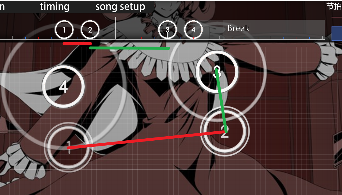
Now let's return to the code analysis part. I believe the most attractive part is the extend velocity, we will draw a graph to explain it
Now please consider Circle 2 as the current object, obviously, the green part is the
curr_vel calculated in the first step, and then, we will enter the if logic.Since the previous object is a slider, the condition is met, and the velocities of the red part and the orange part are then calculated and summed to maximize with the original
curr_vel.Obviously, for this pattern, the sum of the velocities of the red part and the orange part is larger than that of the green part, so the subsequent value is used as the
curr_vel.Objectively speaking, extend velocity is a better representation of the speed of Slider 1 -> Circle 2.
Acute wide angle pattern
In the previous section, we calculated the base value of the strain based on the velocities, and in this section, the algorithm considers the typical acute and obtuse patterning to derive specific bonus.
Note: The code here has been trimmed, reordered and extracted to improve readability without changing the logic.
Here we divide the code into four parts according to the annotations: Rhythm Judgment, Base Calculation, Acute Bonus Calculation, and Repeat Penalty.
// * If rhythms are the same (Rhythm Judgment).
if osu_curr_obj.strain_time.max(osu_last_obj.strain_time)
    < 1.25 * osu_curr_obj.strain_time.min(osu_last_obj.strain_time)
{
    // * Rewarding angles, take the smaller velocity as base (Base Calculation).
    let angle_bonus = curr_vel.min(prev_vel);

    wide_angle_bonus = Self::calc_wide_angle_bonus(curr_angle);
    acute_angle_bonus = Self::calc_acute_angle_bonus(curr_angle);

    // * Only buff deltaTime exceeding 300 bpm 1/2 (Acute Bonus Calculation).
    if osu_curr_obj.strain_time > 100.0 {
        acute_angle_bonus = 0.0;
    } else {
        let base1 =
            (FRAC_PI_2 * ((100.0 - osu_curr_obj.strain_time) / 25.0).min(1.0)).sin();

        let base2 = (FRAC_PI_2
            * ((osu_curr_obj.lazy_jump_dist).clamp(50.0, 100.0) - 50.0)
            / 50.0)
            .sin();

        // * Multiply by previous angle, we don't want to buff unless this is a wiggle type pattern.
        acute_angle_bonus *= Self::calc_acute_angle_bonus(last_angle)
        // * The maximum velocity we buff is equal to 125 / strainTime
            * angle_bonus.min(125.0 / osu_curr_obj.strain_time)
            // * scale buff from 150 bpm 1/4 to 200 bpm 1/4
            * base1.powf(2.0)
                // * Buff distance exceeding 50 (radius) up to 100 (diameter).
            * base2.powf(2.0);
    }

    // * (Repeat Penalty)

    // * Penalize wide angles if they're repeated, reducing the penalty as the lastAngle gets more acute.
    wide_angle_bonus *= angle_bonus
        * (1.0
            - wide_angle_bonus.min(Self::calc_wide_angle_bonus(last_angle).powf(3.0)));
    // * Penalize acute angles if they're repeated, reducing the penalty as the lastLastAngle gets more obtuse.
    acute_angle_bonus *= 0.5
        + 0.5
            * (1.0
                - acute_angle_bonus
                    .min(Self::calc_acute_angle_bonus(last_last_angle).powf(3.0)));
}
Rhythm JudgmentThe rhythm is determined at the top level, so that only objects that meet the criteria will receive the extra bonuses.
First of all, the algorithm ensures that the rhythm change is small, limiting the time change between the current object and the previous object is within 25%.
Objectively speaking, a pattern can only be formed if the rhythm change is small. If the rhythm varies too much, it can't be called as pattern.
Base Calculation
wide_angle_bonus = Self::calc_wide_angle_bonus(curr_angle);
acute_angle_bonus = Self::calc_acute_angle_bonus(curr_angle);

fn calc_wide_angle_bonus(angle: f64) -> f64 {
    (3.0 / 4.0 * ((5.0 / 6.0 * PI).min(angle.max(PI / 6.0)) - PI / 6.0))
    .sin()
    .powf(2.0)
}

fn calc_acute_angle_bonus(angle: f64) -> f64 {
    1.0 - Self::calc_wide_angle_bonus(angle)
}
Then, the algorithm calculates the base values for the wide-angle and acute-angle gains based on the angle between objects. This base value is in the range 0 ~ 1.((5.0 / 6.0 * PI).min(angle.max(PI / 6.0)) - PI / 6.0) Calculate the angle offset from π/6.3/4 * 偏移值 Stretch the domain to (30, 150).sin²(偏移值) Limit results to 0 ~ 1Using GeoGebra, we can draw the following graphs, with the red line representing the wide-angle curve and the blue line representing the acute-angle curve.
Above 30 degrees, the wide angle bonus grows smoothly with the angle. Below 150 degrees, the acute-angle bonus grows smoothly with the angle. Objectively, this is a natural design
Obviously, the algorithm intentionally treats angles below 30 degrees as acute angles and angles above 30 degrees as wide angles, and what we often refer to as right-angle and obtuse-angle patterns actually fall into the realm of wide angles.Acute Bonus Calculation
First of all,
osu_curr_obj.strain_time > 100.0 limits only jumps over 300 BPM or stream over 150 BPM will be bonused in acute-angle bonus, which means that hit object won't get acute-angle bonus in most cases.This is an interesting and logical conclusion. Needless to say, it's hard to jump at 300 BPM or more. Stream over 150 BPM may seem like an easy bonus, but consider this, streams less than 90 degrees require STRONG aim control abilities.
Some readers may have concerns about setting acute_angle_bonus to 0. These concerns will be addressed in the following sections.
In fact, the final bonus is the greater of the acute and wide bonuses**, i.e. an object is considered either wide or acute.
let base1 =
    (FRAC_PI_2 * ((100.0 - osu_curr_obj.strain_time) / 25.0).min(1.0)).sin();

let base2 = (FRAC_PI_2
    * ((osu_curr_obj.lazy_jump_dist).clamp(50.0, 100.0) - 50.0)
    / 50.0)
    .sin();

// * Multiply by previous angle, we don't want to buff unless this is a wiggle type pattern.
acute_angle_bonus *= Self::calc_acute_angle_bonus(last_angle)
// * The maximum velocity we buff is equal to 125 / strainTime
    * angle_bonus.min(125.0 / osu_curr_obj.strain_time)
    // * scale buff from 150 bpm 1/4 to 200 bpm 1/4
    * base1.powf(2.0)
    // * Buff distance exceeding 50 (radius) up to 100 (diameter).
    * base2.powf(2.0);
The comments here greatly facilitate our understanding.*= Self::calc_acute_angle_bonus(last_angle) plays a role in circumventing outliersAs mentioned in the comments, the algorithm only wants to consider wiggly acute angles, which can be understood as several consecutive objects matching the characteristics of acute angle pattern.
While casual and sudden acute is not included in the bonus range, which is reasonable, because it should not be considered as any pattern.
Then, the algorithm scales velocity, strain_time, and distance:
The bonus range of base1: 150 ~ 200 BPM stream (1/4 snapping)
The bonus range of base2: 50 ~ 100 units (center of one circle lies on the circumference of another circle ~ tangent circle)
Repeat Penalty
// * Penalize wide angles if they're repeated, reducing the penalty as the lastAngle gets more acute.
wide_angle_bonus *= angle_bonus
    * (1.0
        - wide_angle_bonus.min(Self::calc_wide_angle_bonus(last_angle).powf(3.0)));
// * Penalize acute angles if they're repeated, reducing the penalty as the lastLastAngle gets more obtuse.
acute_angle_bonus *= 0.5
    + 0.5
        * (1.0
            - acute_angle_bonus
                .min(Self::calc_acute_angle_bonus(last_last_angle).powf(3.0)));
After analysis, we can abstract the key part of the penalty as 1.0 - f(x), where an increase in f(x) implies a larger penalty.Here the repeated wide angle can be penalized by comparing the last bonus.
If last angle is sharper, the penalty factor f(x) will be reduced, thus imposing a lighter penalty on the repeated wide angle
The
min() chooses a smaller value for the penalty factor, to ensure that the penalty factor does not exceed the value of wide_angle_bonus.Velocity Change
In the previous section, the algorithm applied bonus to the acute and wide angle patterns, based on the assumption that the velocities are similar, i.e., the velocity changes are within 25%.
In the following we will introduce the velocity change bonus, which has the opposite assumption from above, i.e., the velocity must be different, and we will analyze it using a similar procedure as in the previous section.
Here we divide the code into three parts: Ratio Calculation, Base Calculation, and Rhythm Change Penalty.
if prev_vel.max(curr_vel).not_eq(0.0) {
    // * (Ratio Calculation)
    // * We want to use the average velocity over the whole object when awarding
    // * differences, not the individual jump and slider path velocities.
    prev_vel = (osu_last_obj.lazy_jump_dist + osu_last_last_obj.travel_dist)
        / osu_last_obj.strain_time;
    curr_vel =
        (osu_curr_obj.lazy_jump_dist + osu_last_obj.travel_dist) / osu_curr_obj.strain_time;

    // * Scale with ratio of difference compared to 0.5 * max dist.
    let dist_ratio_base =
        (FRAC_PI_2 * (prev_vel - curr_vel).abs() / prev_vel.max(curr_vel)).sin();
    let dist_ratio = dist_ratio_base.powf(2.0);

    // * Reward for % distance up to 125 / strainTime for overlaps where velocity is still changing. (Base Calculation)
    let overlap_vel_buff = (125.0 / osu_curr_obj.strain_time.min(osu_last_obj.strain_time))
        .min((prev_vel - curr_vel).abs());

    vel_change_bonus = overlap_vel_buff * dist_ratio;

    // * Penalize for rhythm changes. (Rhythm Change Penalty)
    let bonus_base = (osu_curr_obj.strain_time).min(osu_last_obj.strain_time)
        / (osu_curr_obj.strain_time).max(osu_last_obj.strain_time);
    vel_change_bonus *= bonus_base.powf(2.0);
}
Ratio CalculationBased on
vel_change_bonus = overlap_vel_buff * dist_ratio, we find that the final velocity change bonus is calculated using the base * ratio formula, we will first look at how the ratio is calculated.First, the
prev_vel and curr_vel were recalculated, using the green line of the previous figure as the velocity values.Next,
dist_ratio is calculated in a similar way to the angle bonus above, using sine and then square, and obviously, dist_ratio also takes values in the range of [0, 1].(prev_vel - curr_vel).abs() / prev_vel.max(curr_vel) calculates the ratio of the magnitude of the velocity change to the maximum velocity, reflecting the intensity of the velocity change.The intensity of the velocity change as a ratio of the speed bonus, couldn't be more appropriate!
(a - b).abs() / a.max(b) is a feature scaling method that scales a range of values of arbitrary magnitude into the interval [0, 1].
Here x and y can be considered as the velocity of the current object and the previous object respectively, and the z value is the normalized velocity change.
The sine-then-square approach mentioned twice above is actually a form of feature mapping, where the original value x is mapped to the range [0, 1], and the squaring operation enhances the magnitude of the mapping.Base Calculation
To consider the magnitude of the change, the reader may wish to consider the slope (derivative) of the sine function at each point, and the magnitude of the change will be readily apparent.
Obviously, velocity change is used directly as the base value.
(prev_vel - curr_vel).abs() calculates the difference between the velocities of the before and after objects.(125.0 / osu_curr_obj.strain_time.min(osu_last_obj.strain_time)) limits the influence of distance on velocity.The limit ensures that only velocity changes within a certain range are considered when calculating velocity changes. This makes the bonus value focus more on velocity changes between closer objects and ignore changes between more distant objects.
Rhythm Change Penalty
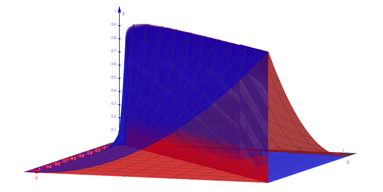
The time-change penalty here uses a similar normalization technique. The value of bonus_base (which is actually interpreted as penalize_base) is in the range [0, 1].
We plot the image of bonus_base, where the x and y axes are the strain_time, and the z axis is the value of bonus_base:
It is clear that when the strain_time is constant, there is almost no penalty (the value of bonus_base is 1).
When there is a change in strain_time, we assume a horizontal and vertical coordinate, there is always a smaller bonus_base corresponding to it. The larger the change in time, the larger the penalty is.
Note: Since the x and y axis of strain_time can be scaled equally, they are set to 1 for easy viewing.It may not be easy for the reader to understand why there is a penalty for time change, so here is an example in the gameplay:
We'll consider Circle 3 to be the current object, and Circle 2 to be the previous object, algorithm will use the velocities of both to calculate the penalty of Circle 3.
The speed of Circle 3 is calculated using the green line, which is a small distance and a long time, so the speed must be very small.
The speed of Circle 2 is calculated using the red line, which is a short time with a large distance, and the speed must be very large.
Without introducing a time-change penalty, the algorithm will consider Circle 3 to be more difficult because of the large velocity change that occurs.
But in fact, in the gameplay, because there is a long time interval between Circle 3 and the previous object, the speed change is no longer felt, and the difficulty of Circle 3 is pretty low at this time.
On the other hand, if we drag the timeline of 1, 2, 3, 4 evenly, then this is a difficult pattern, and the player needs some aim control when hitting Circle 3.
Base *= Bonus
if osu_last_obj.base.is_slider() {
    // * Reward sliders based on velocity.
    slider_bonus = osu_last_obj.travel_dist / osu_last_obj.travel_time;
}

// * Add in acute angle bonus or wide angle bonus + velocity change bonus, whichever is larger.
aim_strain += (acute_angle_bonus * Self::ACUTE_ANGLE_MULTIPLIER).max(
    wide_angle_bonus * Self::WIDE_ANGLE_MULTIPLIER
        + vel_change_bonus * Self::VELOCITY_CHANGE_MULTIPLIER,
);

// * Add in additional slider velocity bonus.
if with_sliders {
    aim_strain += slider_bonus * Self::SLIDER_MULTIPLIER;
}

aim_strain
In the above section, we have calculated the various bonus and base values needed for the final calculation, and it is finally time to finalize the aim_strain calculation.The first thing we see in the code are some defined constants (in all caps and underlined), which specify the proportion of each bonus in the final calculation.These constants reflect the weights of the parameters involved in the final calculation
Besides the constants, there are a couple of calculations, the first being the slider bonus calculation, which is rather simple:
Slider Distance / Slider Time.This type of slider bonus will mainly be applied to beatmaps with long, high speed sliders (like Genryuu Kaiko).
Also, the way
aim_strain picks up acute, wide and speed bonus is quite interesting . it uses the larger one of acute or wide + speed.As we mentioned above, the conditions for applying acute bonus are very tough (300 BPM jumps, 150 BPM streams), which means that most of the objects will not get the acute bonus.
Looking at the values of the constants, we see that the multiplier for acute bonus is larger than the multiplier for wide bonus, which provides higher rewards for more difficult and demanding patterns.
Simply speaking, most of the object bonus comes from the Wide Angle + Speed formula, and those common beatmaps don't even have a chance to get any Acute Angle bonus.
Explore Speed
Similar to Aim, let's first focus on the ISkill implementation of Speed in speed.rs, focusing on the
strain_value_at method.fn strain_value_at(&mut self, curr: &'a OsuDifficultyObject<'a>) -> f64 {
self.inner.curr_strain *= strain_decay(curr.strain_time, STRAIN_DECAY_BASE);
self.inner.curr_strain +=
SpeedEvaluator::evaluate_diff_of(curr, self.diff_objects, self.inner.hit_window)
* SKILL_MULTIPLIER;
self.inner.curr_rhythm =
RhythmEvaluator::evaluate_diff_of(curr, self.diff_objects, self.inner.hit_window);
let total_strain = self.inner.curr_strain * self.inner.curr_rhythm;
self.inner.object_strains.push(total_strain);
total_strain
}After a skimming, we discovered a slight difference with the Aim calculation above. Here curr_strain(speed_strain) is used as the base value, and curr_rhythm is used as the factor. Obviously, the speed is multiplied by the rhythmic complexity as the final value, therefore we divide the calculation into two main sections: SpeedEvaluator and RhythmEvaluator.The Rhythm Complexity (RhythmEvaluator) here is the concept introduced in November 2021 Rework by Xexxar.
The Rework was controversial and highly publicized, yet it somewhat prevented Aim from becoming the main way to get PP, and brought osu! back from being a gopher simulator. We'll focus on that part later.
History on the development of rhythmic complexity:Next, we'll go through each piece of the code one by one, in the same order as the code.
abraker95 had proposed a theory of rhythmic complexity in 2019: On the topic of rhythmic complexity
2019, Community Understanding and Discussion for Rhythmic Complexity: Rhythmic Complexity
SpeedEvaluator
Before we start introducing SpeedEvaluator, let's expand on some concepts:
hit_window: The window of time during which the hit should be completed, and is closely related to the OD of the beatmap (note that all references to the hit_window in rosu-pp are to the entire hit_window, which is calculated as two times larger).The hit window (in ms) can be seen in-game by hovering the cursor over the 3D position of the beatmap in the upper-left corner. osu!standard mode calculates it like this.
Recommended reading of osu!Wiki: Overall difficultySingle tap? Doubled!
Algorithms always need to be iteratively updated to follow the mapper's talent, and innovative beatmaps can often push PP systems to update, this is how doubletapness was introduced
The introduction of doubletapness comes from the beatmap below:
It should be noticeable that there are several single beats in the segment that require double-tapping, which, in Speed calculations, is judged to be an extremely high-speed cut, and what's more, this will be exacerbated by the DTHR.
Before the introduction of doubletapness, this map was given a super-high 13 stars after DTHR (currently 8.66)
// * Nerf doubletappable doubles.
if let Some(osu_next_obj) = osu_next_obj {
    let curr_delta_time = osu_curr_obj.delta_time.max(1.0);
    let next_delta_time = osu_next_obj.delta_time.max(1.0);
    let delta_diff = (next_delta_time - curr_delta_time).abs();
    let speed_ratio = curr_delta_time / curr_delta_time.max(delta_diff);
    let window_ratio = (curr_delta_time / hit_window).min(1.0).powf(2.0);
    doubletapness = speed_ratio.powf(1.0 - window_ratio);
}
window_ratio compares two neighboring objects to a hit_window of 300. Assuming N is the current object, if delta(N, N-1) is smaller than the hitwindow of 300, then it can be assumed that there is doubletapness between (N-2, N-1) and (N-1, N), where window_ratio is a qualitative indicator of doubletapness.The
delta_diff indicates the difference between the current interval and the next interval. Here we take any Circle 2 in the GIF as an example, the value of Circle 2 will be very large (2 is very short from the previous 1, and very long from the next 1), and if we look at any Circle 1, we can get the same conclusion. Here we find that delta_diff is a quantitative indicator of doubletapness.The
speed_ratio is part of the decay amplitude. The purpose is to normalize raw_doubletapness to the current dimension.The hitwindow of 300 mentioned here can be calculated using the formula above:Note that around 2021, apollo-dw promoted many proposals related to Speed calculations, and doubletapness is just a rainy day for apollo-dw's great reforms.2(80 - 6 * OD), where 2 means that we consider the whole hitwindow, including positive and negative ones.
doubletapness was introduced by apollo-dw in 2022: Rework doubletap detection in osu!'s Speed evaluator
You can go to the graphing calculator provided by apollo-dw and try to adjust the parameters yourself.: Desmos
apollo-dw's name will also appear below.
Velocity & Distance
// * Cap deltatime to the OD 300 hitwindow.
// * 0.93 is derived from making sure 260bpm OD8 streams aren't nerfed harshly, whilst 0.92 limits the effect of the cap.
strain_time /= ((strain_time / hit_window) / 0.93).clamp(0.92, 1.0);
// * derive speedBonus for calculation
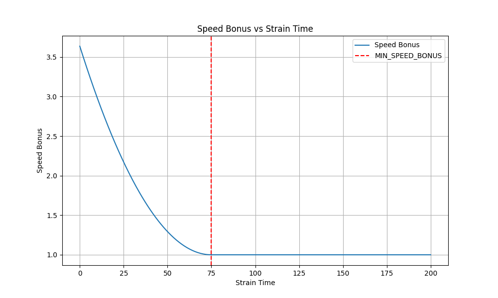
let speed_bonus = if strain_time < Self::MIN_SPEED_BONUS {
let base = (Self::MIN_SPEED_BONUS - strain_time) / Self::SPEED_BALANCING_FACTOR;
1.0 + 0.75 * base.powf(2.0)
} else {
1.0
};
let travel_dist = osu_prev_obj.map_or(0.0, |obj| obj.travel_dist);
let dist = Self::SINGLE_SPACING_THRESHOLD.min(travel_dist + osu_curr_obj.min_jump_dist);
(speed_bonus + speed_bonus * (dist / Self::SINGLE_SPACING_THRESHOLD).powf(3.5))
* doubletapness
/ strain_timeAt the beginning of the calculation, we note this limitation on strain_time, which is actually derived from a commit in apollo-dw: Remove speed caps in osu! difficulty calculationThe intent of limiting
strain_time is to prevent high BPM low OD streams from getting too high difficulties, as well as to remove the old algorithm's behavior of simply capping the Speed value.It takes into account whether the time between objects is less than 300 hit window, and if it is less, it will nerf the strain_time.
apollo-dw and emu1337 advancedRemove speed caps in osu! difficulty calculation.The speed_bonus starts at 75ms (200BPM), the dist starts at 125 osu!pixel, and the overall trend is that the higher the speed, the farther the distance, the larger the strain value will be.
In the year 2024, these proposals appear to be very forward-thinking, with the advent of wooting dramatically increasing the ability of top players to stream at high speeds, and the removal of the old ~333bpm 1/4 will somehow always be approved.
Here we have graphed
speed_bonus about strain_time using matplotlib:The calculation of dist is very similar to the concept of velocity extends in Aim, so let's reintroduce the image here:
Please consider Circle 2 as the current object, the dist of Circle 2 is the sum of the red and orange distances.
RhythmEvaluator
Since RhythmEvaluator is quite complex, we will first explain the theory in general and then analyze it with the code.
First of all, the RhythmEvaluator itself is the same as the AimEvaluator and SpeedEvaluator above, it is a strain-like value evaluated for a single hit object.
The rhythmic complexity is based on the parameter
effectiveRatio. First, effectiveRatio gets a base value from the initial rhythm change, and then it is reduced in a way similar to intergroup evaluation.Intergroup Evaluation
Now, we use pseudo-code to simulate the process of intergroup evaluation:
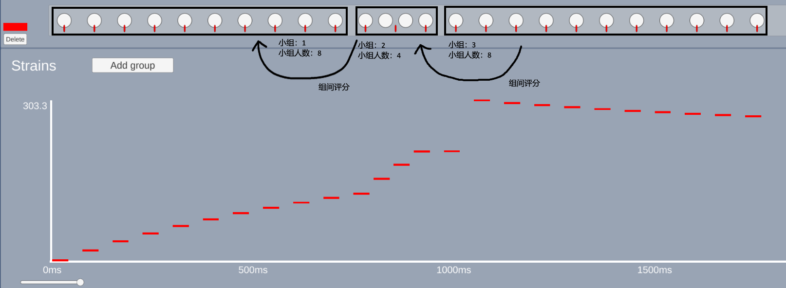
Firstly, find 0~32 history objects of the current object within 5s, and then find the number of matched objects called
rhythmStart.Next, we traverse the history objects sequentially, trying to group the neighbor objects as
island on basis of large change in rhythm (deltaTime changes by more than 25%).After traversing, all historical objects should be organized into groups (
island) of 1 to 8 people. Groups can contain more than 8 objects, but the number of people in the group will only be counted as 8.At last, we have to score between groups (
island), the effectiveRatio value will be reduced when certain patterns appear, for example: groups with equal length are repeating (xxx-xxx), neighbor groups have the same odevity (xx-xxxx), and so on.Diagram (Image partly from emu1337's screenshot):
Realization details
Next, we will analyze the mentioned intergroup evaluation process along with the code. Note that the C# version of the code has been used here in order to improve readability.
Filtering Objects
int historicalNoteCount = Math.Min(current.Index, 32);
int rhythmStart = 0;
while (rhythmStart < historicalNoteCount - 2 && current.StartTime - current.Previous(rhythmStart).StartTime < history_time_max)
    rhythmStart++;
Here rhythmStart, which is not new to us, performs the task of finding the current object within 5s of 0~32 historical objects.Grouping
for (int i = rhythmStart; i > 0; i--)
{
    // (The calculation of the initial value of effectiveRatio is omitted.)

    if (firstDeltaSwitch)
    {
        if (!(prevDelta > 1.25 * currDelta || prevDelta * 1.25 < currDelta))
        {
            if (islandSize < 7)
                islandSize++; // island is still progressing, count size.
        }
        else
        {
            // (The calculation of the reduction of the effectiveRatio has been omitted.)

            /*
                rhythmComplexitySum += Math.Sqrt(effectiveRatio * previousRatio) * currHistoricalDecay * Math.Sqrt(4 + islandSize) / 2 * Math.Sqrt(4 + previousIslandSize) / 2;
                previousRatio = effectiveRatio;
            */

            previousIslandSize = islandSize; // log the last island size.

            if (prevDelta * 1.25 < currDelta) // we're slowing down, stop counting
                firstDeltaSwitch = false; // if we're speeding up, this stays true and we keep counting island size.

            islandSize = 1;
        }
    }
    else if (prevDelta > 1.25 * currDelta) // we want to be speeding up.
    {
        // Begin counting island until we change speed again.
        firstDeltaSwitch = true;
        previousRatio = effectiveRatio;
        islandSize = 1;
    }
}
The code snippet here omits some of the calculation of the values, so that we can focus on the basis of island's grouping.First, the loop lets us iterate over all the history objects, and obviously,
firstDeltaSwitch is the qualitative indicator for the creation of a new island.Once
prevDelta > 1.25 * currDelta is met, i.e. the deltaTime has changed by 25%, the algorithm thinks it is time to create a new island.In the next loop, since
firstDeltaSwitch is set to true, the algorithm will go to the first "if" branch.Obviously, the second if branch determines the grouping result, and once the condition
prevDelta > 1.25 * currDelta || prevDelta * 1.25 < currDelta is met, i.e., a large change in velocity has occurred, the current group will be terminated and settled ("else" branch).The settlement process is the intergroup evaluation we mentioned above. Unlike the pseudo-code description, in the real code, the grouping is done back-to-back with the settlement, rather than grouping and then settling.
Obviously, we're intentionally storing some previousIsland state at settlement time, which, unsurprisingly, creates context for the next group settles.
In addition,Base Calculationif (prevDelta * 1.25 < currDelta) firstDeltaSwitch = false;islands can be created one after another while the velocity maintains an upward tendency. When the velocity is no longer increasing, the qualitative criterion is restored until the next timeprevDelta > 1.25 * currDeltais met.
You may notice an error in our diagram above, in fact, the monotonous rhythms are not divided into one large group, but into many groups with one member.
double currHistoricalDecay = (history_time_max - (current.StartTime - currObj.StartTime)) / history_time_max; // scales note 0 to 1 from history to now

currHistoricalDecay = Math.Min((double)(historicalNoteCount - i) / historicalNoteCount, currHistoricalDecay); // either we're limited by time or limited by object count.

double currRatio = 1.0 + 6.0 * Math.Min(0.5, Math.Pow(Math.Sin(Math.PI / (Math.Min(prevDelta, currDelta) / Math.Max(prevDelta, currDelta))), 2)); // fancy function to calculate rhythmbonuses.

double windowPenalty = Math.Min(1, Math.Max(0, Math.Abs(prevDelta - currDelta) - currObj.HitWindowGreat * 0.3) / (currObj.HitWindowGreat * 0.3));

windowPenalty = Math.Min(1, windowPenalty);

double effectiveRatio = windowPenalty * currRatio;
currHistoricalDecay
In the Grouping section of the code presentation, we skipped over the calculation of the
rhythmComplexitySum, which referenced the concept of currHistoricalDecay.Revisiting the whole process, we will apply the RhythmEvaluator to each object. It is dangerous to put the effect of sum value in a single object, and we need to spread the sum influence over the strains in each objects.
The simplest way would be to divide
rhythmComplexitySum by rhythmStart, but this is obviously not wise. So here we introduce currHistoricalDecay.The
currHistoricalDecay scales uniformly according to the difference in time, spreading the sum over 0 to N historical objects.effectiveRatio
The expression of
currRatio is not new to us. The
currRatio function (sine then square) is not new to us, and is exactly the same as the velocity change bonus mentioned in Aim.(prev_vel - curr_vel).abs() / prev_vel.max(curr_vel)calculates the ratio of the magnitude of the velocity change to the maximum velocity, reflecting the intensity of the velocity change.
Similarly, the normalization of the factors is done in a sine-then-square approach, and the reader can check back above if needed.
Xexxar has also put up a graphing calculator for the formula: Desmos
windowPenalty penalizes overlapping windows, similar to apollo-dw's doubletapness.Intergroup Calculations
if (currObj.BaseObject is Slider) // bpm change is into slider, this is easy acc window
    effectiveRatio *= 0.125;

if (prevObj.BaseObject is Slider) // bpm change was from a slider, this is easier typically than circle -> circle
    effectiveRatio *= 0.25;

if (previousIslandSize == islandSize) // repeated island size (ex: triplet -> triplet)
    effectiveRatio *= 0.25;

if (previousIslandSize % 2 == islandSize % 2) // repeated island polartiy (2 -> 4, 3 -> 5)
    effectiveRatio *= 0.50;

if (lastDelta > prevDelta + 10 && prevDelta > currDelta + 10) // previous increase happened a note ago, 1/1->1/2-1/4, dont want to buff this.
    effectiveRatio *= 0.125;
Through the codes, it was easy to see the logic of the reduction among the groups. We came to realize the advantages and feasibility of rhythmic grouping.So far, we have explored the design logic and implementation of osu! algorithm through AimEvaluator and SpeedEvaluator. In the process of exploration, I hope that readers can satisfy their curiosity and at the same time gain some simple understanding of the algorithmic system of rhythm games. In this paper, we also involve such statistical knowledge as function fitting, normalization, etc., and I hope that it will help to inspire readers to carry out mathematics-related research.
2024-07-01 to 2024-09-19, Written by TuRou.
2024-09-20 to 2024-09-23, English by TuRou.